
Step 1: Copy the chart as a static image
Press the [shift] key, click the chart area, execute the [Edit - Copy Image] command, and the [Copy Image] dialog box will pop up, press OK.
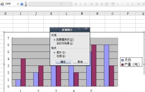
Right-click on a blank cell and paste, and a picture will be copied.
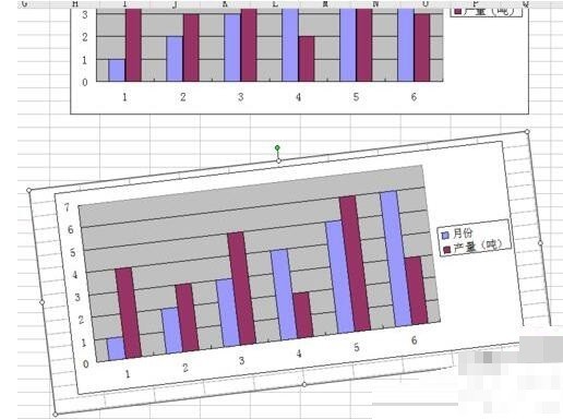
Click the green rotation button above the picture, the mouse pointer will turn into a rotating arrow, and then you can rotate the picture arbitrarily.
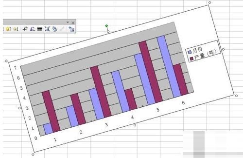
Step 2: Use the camera function
Execute the [View - Toolbar - Customize] command, the [Customize] dialog box will pop up, and then execute [ Command - Category], find [Tools], and then find [Camera] in [Command] on the right.
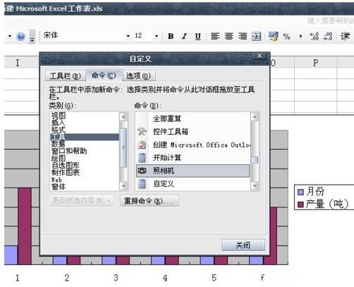
Click the [Camera] icon, left-click and drag the icon out, and add [Camera] to the common toolbar.
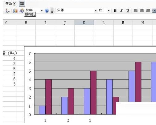
Select the area where the chart is located, in the example it is the H5-Q21 area, and then click the [Camera] command in the toolbar. At this time, the mouse will turn into a cross and a rectangle will appear. area, drag it to a blank space, and a similar picture will appear.
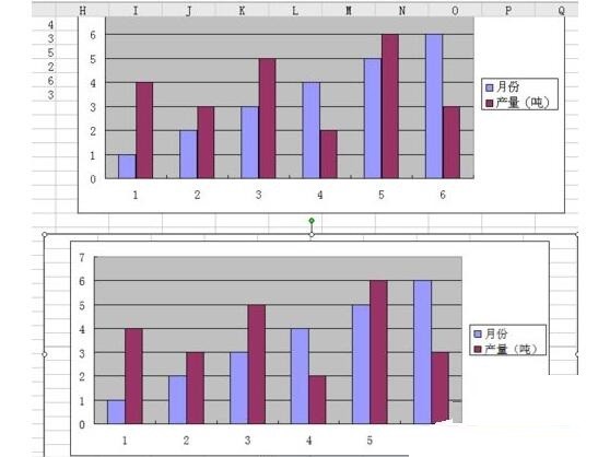
Resize the image to fill the empty space. Click the green rotate button above the picture, the mouse pointer will turn into a rotating arrow, and then you can rotate the picture arbitrarily.
Notes
The picture obtained by the first method is a static picture, and the picture will not change when the chart changes.
The second type is that if the chart in the cell changes, the picture in the rectangle will also change.
The above is the detailed content of Detailed tutorial on rotating charts in Excel. For more information, please follow other related articles on the PHP Chinese website!


