In the previous article " Sharing practical Excel skills: How to make bar charts more vivid! 》, we learned about ways to make excel bar charts more vivid and distinctive. Today we will take a look at how to make a smart attendance sheet, come and learn!
If the attendance machine is not so smart and requires manual auxiliary statistics, and if the company has not yet used an attendance machine, making the attendance sheet for the current month is a complex and lengthy process. Therefore, how to improve work efficiency and complete monthly attendance statistics within a limited time is a big deal for the MM in the personnel department.
To improve efficiency, you must have a better attendance sheet. This attendance sheet must have at least the following points:
Simplify input of attendance items
Display weekend data prominently
Can automatically summarize data
Today the old rookie will teach you how to make a smart attendance sheet that has the above three points at the same time. Come and take a look!
Before you start making it, let’s take a look at the final effect display:
In the demonstration, you can find the following points:
Title input is very simple, you only need to enter a month number;
The number of days in the month will automatically change, and the date will automatically adjust and display according to the month. At the same time, Saturday and Sunday It will change color automatically;
Use the drop-down menu to complete the input of attendance data, and there will be prompt information;
There is an attendance result statistics area on the right side of the form. Statistical data is automatically generated based on the filled-in content.
Let’s teach you how to make such a form.
1. Production of the main body of the attendance sheet
First, make a basic form, as shown in the figure:
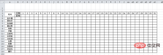
The method of making this form is very simple. I believe everyone can complete it. The next step is a little detail work, so be sure to read it carefully.
Merge the first row, and the last five cells of the second row, merge three and two respectively. The finished effect is as shown below:

Right-click on the merged cell in the first row and select "Format Cells". In the pop-up dialog box, the customized format is: Xinsheng Company Attendance Statistics Table for October.
#Note that this is the number 0, not the letter O.
After the settings are completed, click OK, then enter a number in the first line to see the effect.
#Isn’t it amazing? In fact, this is the use of the characteristics of custom formats.
Just enter the "number of days in the month" in the second line directly, followed by the formula: =DAY(EDATE(DATE(2018,A1,1),1)-1)
Let me briefly introduce the meaning of this formula. Three date functions are used:
The format of the DATE function is: DATE (year, month, day) , that is, get a date based on the specified year, month and day. In this example, the year is 2018 (if it is the next year, just change it to 2019), the month is the number entered in the first line, and the day is 1. The date obtained in this way is the 1st of the month of the attendance sheet.
The format of the EDATE function is: EDATE (start date, number of months apart), that is, a new date is obtained based on the specified date and the number of months apart. The start date in this example is The 1st of the current month, and the number of months apart is 1, indicating the date of the 1st of the next month.
The format of the DAY function is: DAY (date), to get the day of the month for the specified date. In this example, the specified date is one day before the 1st of the next month (after the EDATE function There is minus 1), in other words, it is the last day of the month. Then use the DAY function to get the total number of days in the month.
Note: Date functions are often used together with several functions, and there are many ways to think about the same problem. Some formulas have very clever ideas, which is also the fun of learning functions. one.
The next thing to set is the week. Fill in the formula in cell C4: =TEXT(DATE(2018,$A1,C3),"aaa"), and drag it to the right.
Formula=TEXT(DATE(2018,$A$1,C$3),"aaa") uses two functions TEXT and DATE. Explain the functions of these two functions respectively:
The DATE function has just been mentioned. In this formula, the year is still 2018, and the month is A1. Because the formula needs to be pulled to the right, in order to prevent A1 from changing when pulling to the right, add in front of the column number After $ is locked, the day is represented by the number corresponding to the third line, so that all the dates of the month are obtained.
The format of the TEXT function is: TEXT (data to specify the format, format code). This function is considered a relatively advanced function. Although the structure is relatively simple, it has a lot of format codes, so it is also a multi-functional function. The format code in this example is "aaa", which uses one word to display the day of the week. Interested readers can try the effects of the codes "aaaa", "ddd" and "dddd" respectively.
Note: When using the TEXT function, the format code must be enclosed in quotation marks (the quotation marks are entered in English mode).
At this point, the table is basically completed. Some units may not distinguish between morning and afternoon, but some units do. How to change one row for each person into two rows? Is it possible to insert one row at a time? ? Definitely not. A very simple trick is used here. Let’s take a look through the animation demonstration:
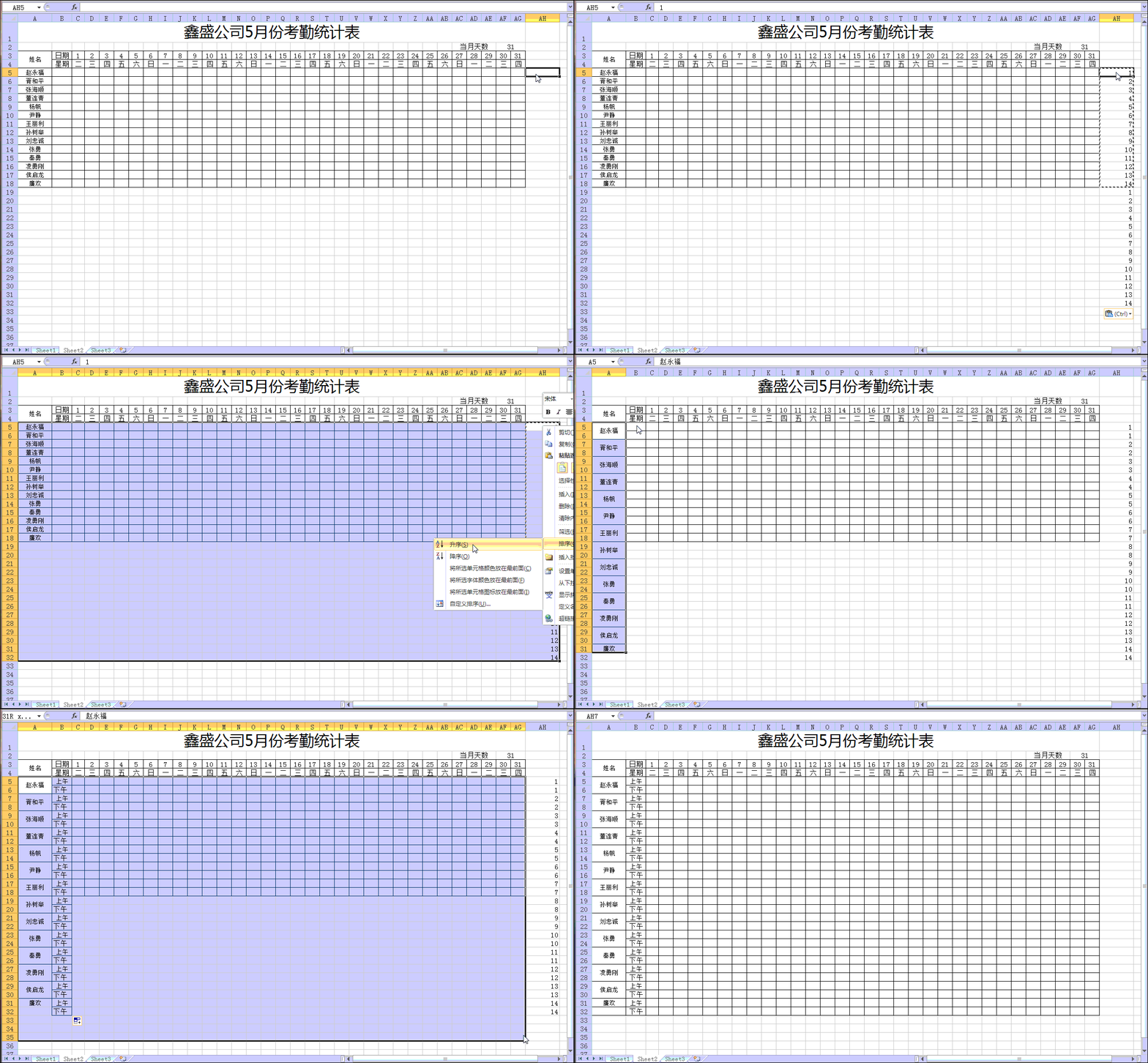
In this operation, several techniques are involved: batch insertion I hope you can practice more and become proficient in the techniques of blank lines, techniques of using the format brush, and techniques of quickly filling in repeated content.
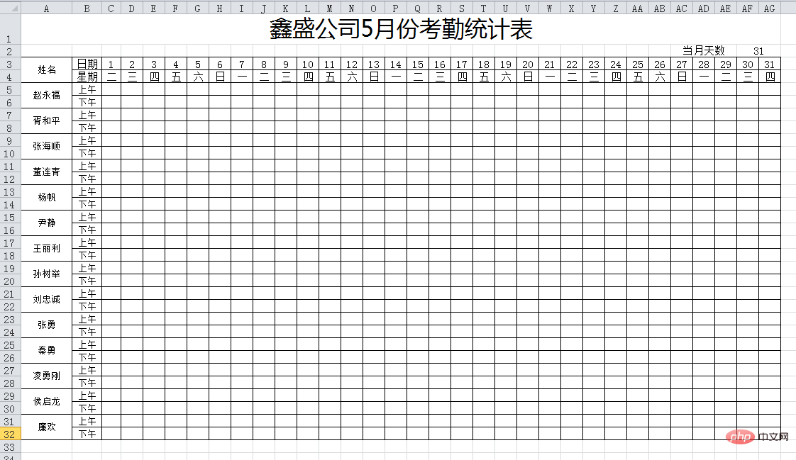
At this point, the theme of this attendance sheet has been prepared, and the effect is as follows:
2. Use conditional formatting and Data validity processing table
The next two tasks need to be completed:
Let the dates in the table be displayed according to the actual situation, and at the same time, Saturday Sunday will automatically change color;
Attendance data is entered using the drop-down menu, and there is a prompt message.
Let’s see how to achieve these effects. For the first item, you need to use the conditional formatting function. Although there are not many steps, there are many details. Please follow them slowly:
(1) Select the data area and click [Conditional Formatting]-[ New rule]:
Further select [Use formulas to determine the cells to be formatted] and enter the formula: =C$3>$AF$2 , and then click the [Format] button:
Formula analysis: Very simple, it is to compare whether each date in the third line is greater than the number of days in the month. If If it is large, execute it according to the set format. Pay attention to the position of $ in this step.
Select [Custom], enter three semicolons in the type:;;;, pay attention to the semicolons in English state, and click OK after completion.
Format code explanation: The specific meaning is more complicated. Remember Entering three semicolons means not displaying the content of the cell.
Click OK again. At this time, you can find that the data that does not belong to the date of the current month can no longer be seen:

Further set Saturday and Sunday Automatically change color, or select the data area, create a new rule, enter the formula =OR(C$4="six",C$4="day") and set the format:
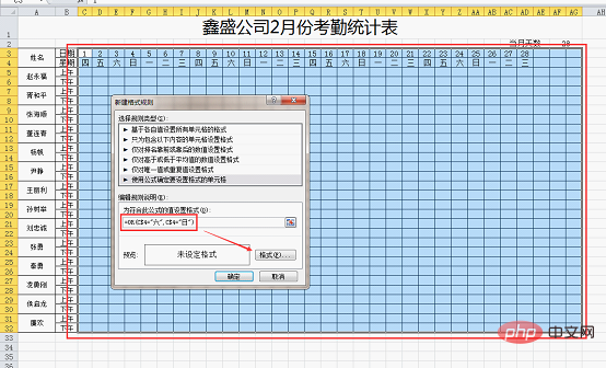
this The formula is also easy to understand. If OR meets either of the two conditions, it will be executed according to the set format. That is, if the fourth line is "six" or "day", the specified color will be displayed.
After clicking the Format Cells button, select [Fill], select a color, and click OK.
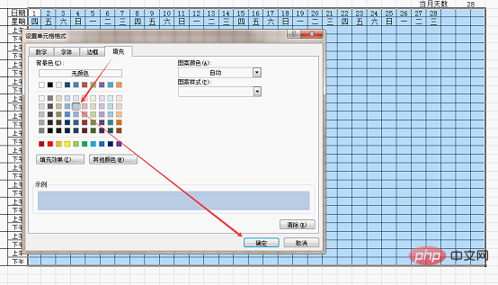
Click OK again to see the effect:
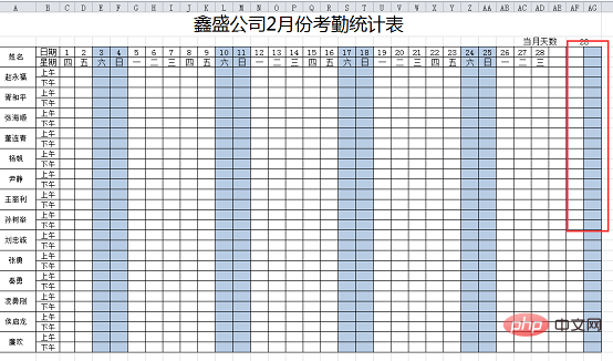
Hey, why are the empty spaces at the back also colored? What went wrong?
Looking carefully, I found that this place happened to be Saturday, but it was hidden by the format set previously, but it still took effect when coloring. How to deal with this problem? It's very simple. After selecting the data area, open the management rules of conditional formatting:
#Tick "Stop if true" after the following rule, and then click the Move Up button , click OK.
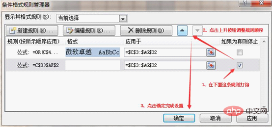
See the effect?
Next, we need to set the validity of the attendance data. Before proceeding with this step, let us first complete the creation of the statistical area.
3. Production of statistical area
The production of this area is very simple. According to your actual needs, add a remarks column. Fill in the attendance items and legend, and use the COUNTIF function under each legend to complete statistics. The formula is =COUNTIF($C5:$AG6,AI$4)/2:
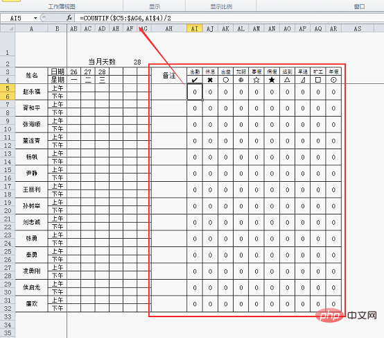
The format of the COUNTIF function is: COUNTIF (statistical area, content to be counted). In layman’s terms, it is the appearance of each attendance item (content to be counted) in the two rows (statistical area) corresponding to each person. times, because the daily data in the example is two rows, so the statistical result must be divided by 2.
As for the processing of these merged cells, it is very simple. Just merge one and then use the format brush to brush it.
Now go back and set the drop-down menu of attendance data. Before setting the validity, do some preparation work first, copy the legend and description for later use, and then set the validity. Let’s watch the animation demonstration for this part of the operation:
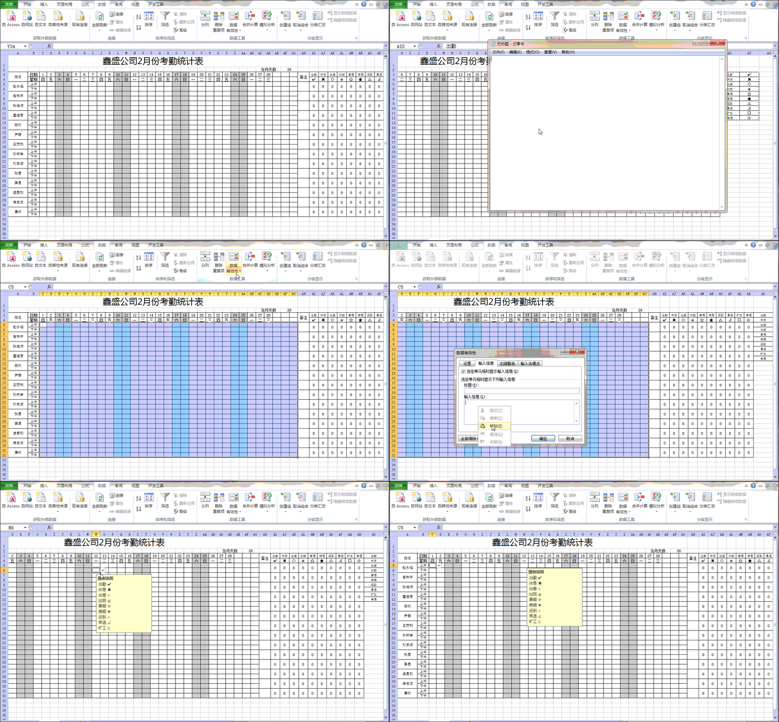
At this point, the attendance sheet is completed. I believe you will gain a lot from today’s content!
Related learning recommendations: excel tutorial
The above is the detailed content of Practical Excel skills sharing: Make a smart attendance sheet. For more information, please follow other related articles on the PHP Chinese website!
 Compare the similarities and differences between two columns of data in excel
 excel duplicate item filter color
 How to copy an Excel table to make it the same size as the original
 Excel table slash divided into two
 Excel diagonal header is divided into two
 Absolute reference input method
 java export excel
 Excel input value is illegal