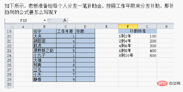
In the previous article " Practical Excel skills sharing: learn how to make a multi-factor ranking statistical table? 》, we learned about how to make a multi-factor ranking statistical table, and today we are going to talk about citations in Excel formulas. Don’t you understand absolute citations and mixed citations? No wonder you always fill in the wrong formulas!
Let me analyze this question for you.

After reading everyone’s comments, I found that there is a common problem with everyone’s formulas: the first parameter of each nested IF function uses the AND function to specify the data. range.
For example:
Also like this:
No matter whether the above formula is Correct, think about it, do we need to write so many ANDs?
Perhaps everyone was influenced by the tutorial - who said this tutorial just exemplified the AND function, and who said the subsidy years could just be described by AND? Haha...
(In the last question, due to the carelessness of the bottle, I forgot to write down the subsidy for more than 10 years! I will punish myself by writing more tutorials, so now we will unify that the subsidy for more than 10 years is also 600) There are two ways to write the
formula. The first one is:
=IF(C:C
When the number in column C is less than 1, return 0, otherwise Just look at the second IF directly. At this time, the default is greater than or equal to 1, so the second IF only needs to write the upper limit of the number, which is less than 2. The following is the same.
The above formula limits all upper limits. In fact, it can also limit all lower limits. The second type:
=IF(C:C>=8,600,IF(C:C> ;=6,400,IF(C:C>=4,300,IF(C:C>=2,200,IF(C:C>=1,100,0)))))
When column C When the number is greater than or equal to 8, it returns 600, when it is greater than or equal to 6, it returns 400, when it is greater than or equal to 4, it returns 300, when it is greater than or equal to 2, it returns 200, when it is greater than or equal to 1, it returns 100, otherwise it returns 0.
You can find that if you use IF to answer this question, use the second method and set the lower limit of the data every time, which is easier to understand.
In addition, Bo Bo also wants to tell you that when entering formulas in the edit bar, sometimes you don’t have to enter them manually. For example, in the above formula, we directly click on column number C, and it will appear in the formula. C:C. The formula written by the second friend above uses absolute reference. You can also directly drag and select the data area B5-B14 and press F4, and it will become $B$5:$B$14.
Maybe those who are just getting started don’t know much about relative references and absolute references. Today Bottle will explain them to you.
1. Relative reference
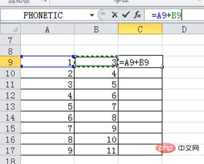
As shown below, the data in columns A and B are summed, and the summation result is displayed in column C. .
As shown below, after selecting cell C9, enter the equal sign in the edit bar, then directly click on cell A9, enter the plus sign, and then directly click on cell B9. Finally enter.

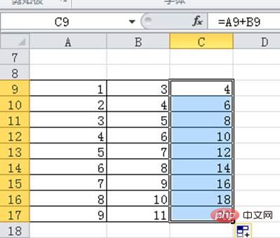
Select cell C9, place the mouse in the lower right corner, double-click, and you can see that the entire column has been summed.

At this time, we click on the cells in column C one by one, and we can see the formula in the edit bar. As we move down, the row number will also change. Change to the corresponding line number.
You can try entering the formula in cell A18, summing column A, and drag the fill formula horizontally to cell C18. . You will see that when you drag the formula horizontally, the column number will automatically change to the corresponding column number. This is called a relative reference. The relative reference format of a cell is the column number and row number. For example, A10, B14, etc. are all relative references. The biggest feature of relative references is that when you drag to fill in a formula, the cell will automatically change based on the location of the formula.
2. Absolute reference
What is an absolute reference?
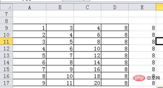
As shown in the figure below, select cell D9, enter =sum(), click in the square brackets, directly drag to select A9-C9, then press F4, and finally press Enter.
At this time, double-click to fill in the formula, and then click on each cell in column D to view the formula. You will find that the formulas in the entire column are exactly the same. What is the difference between
and relative reference? The difference is that the row number and column number referenced in the current formula are preceded by the "$" symbol. $ is a "lock" that locks the cell, so no matter we pull it horizontally or vertically, the formula will not change in any way. This is called an absolute reference.
3. Mixed Reference
In the previous formula, the row number and column number are both "locked", but think about it, When filling in the formula vertically, the column number will not change even if we do not lock the column number.
As shown below, in cell E9, after entering =sum(), click in the square brackets, drag and select the cell range A9-C9, and then press F4 twice. At this time, only the rows are locked. Number.
After double-clicking to fill down, you can see that the result is exactly the same as the previous absolute reference result.

This kind of operation that only locks the row number or column number is called a mixed reference. Mixed means that cell references include both absolute references and relative references. For example, $A1 means that the column number of the cell is an absolute reference and the row number is a relative reference. The trick to mixed references is: pull down to lock only the row number, and pull to the right to lock only the column number. This way the formula will not change during the dragging process.
It’s time to verify everyone’s learning results!
Look at the table below. The corresponding columns and rows need to be displayed in cells B2-E5. The bottle has set the formula in cell B2. Now think about it, in the formula How to "lock" the row number and column number so that the entire area can be filled in at once?

Leave your answer in the comment area below!
Related learning recommendations: excel tutorial
The above is the detailed content of Practical Excel skills sharing: help you understand 'absolute reference' and 'mixed reference'. For more information, please follow other related articles on the PHP Chinese website!
 Compare the similarities and differences between two columns of data in excel
 excel duplicate item filter color
 How to copy an Excel table to make it the same size as the original
 Excel table slash divided into two
 Excel diagonal header is divided into two
 Absolute reference input method
 java export excel
 Excel input value is illegal


