Practical Excel skills sharing: How to sum data with units?

In the previous article "The magical AGGREGATE of Excel function learning, one can actually be worth 19! 》, we learned about a powerful statistical function. Today we are going to talk about data processing. It turns out that numbers plus units can be summed. Take a look, you must not know this method!

In daily work, when we use function formulas to sum data, the data has no units, so we can easily complete the data sum. However, according to our habits, There should be a unit behind the data. How to sum such data?

1. Common units of data

In the material collection registration form, we are used to writing the unit after the data, such as 12, 15 This class. In Excel, when text is added to a number, it becomes text and cannot be summed directly.

In the table shown in the figure below, SUM cannot be used to sum the "numeric text" data in column F directly.

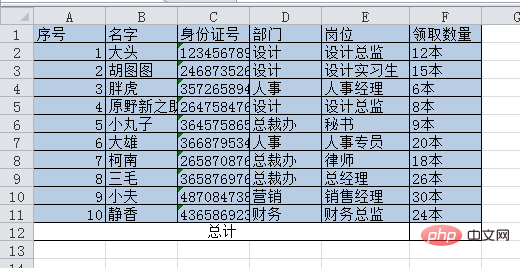
Can you solve it?

Let me introduce 3 methods to you. If you have a better and easier method, please leave a message to share!

The first method: column separation method

We can use the data column method to remove the word "本".

(We have previously discussed data classification in a special tutorial, click to view: //m.sbmmt.com/topic/excel/491825.html)

Select the data in column F, click "Data" - "Column" - "Separator", you can see the dialog box as shown below.

When the delimiter symbol is used as the basis for column classification, the corresponding symbol will become a dividing line, so here, we can turn "this" into a dividing line. Check "Others" and enter "this" next. In the data preview below, you can immediately see that "this" has become a dividing line.

Click Finish. There are only numbers in the data.

Select the data area in column F, click "Formula" - "Automatic Sum" - "Sum" to complete the sum.

(We have a special tutorial on automatic summation before, click to view: //m.sbmmt.com/topic/excel/491692 .html)

Second method: Replacement method

In the previous tutorial, I told you that the find and replace tool can delete characters in batches. We can also use it here. this way.

(To find and replace partners who are still unclear, you can click on the link to view: //m.sbmmt.com/topic/excel/491928.html)

Select the data area in column F and press the replace shortcut key CTRL H. In the pop-up dialog box, enter "this" in "Find content" and do not enter any characters after "Replace with".

Click "Replace All", all "this" in column F will be deleted, and then perform the same summing operation as before.

The third way to open your mind: Custom format method

The first two methods are to remove "this" The data is summed after the word, so is there any way we can sum it without deleting the word "this"? Of course!

Select the data area and first use any of the previous methods to remove the word "本".

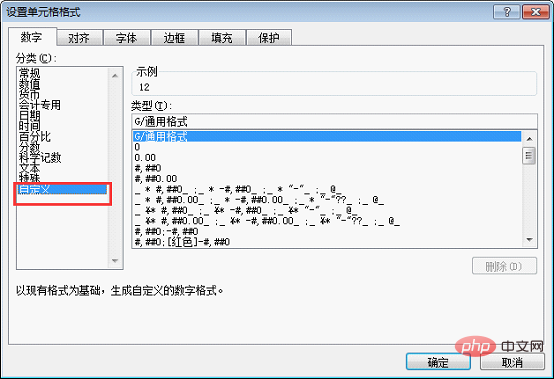
Keep the data selected, then press the ctrl 1 shortcut key to pop up the "Format Cells" dialog box, and click "Customize".

Select "G/General Format" as the type, and then enter the word "this" after "G/General Format". The "G/general format" here means that the data is regular data. Adding the word "Ben" at the end only adds a character to the data and does not change the format of the data.

After clicking OK, there will be the unit "Ben" after the number. The data at this time is aligned to the right, indicating that it is regular data rather than text, while the original data at the beginning of the article is aligned to the left, indicating that it is text. (Data is on the right, text is on the left.)

Let’s verify it to see if it can be summed.

Same as the previous operation, after selecting the data, click "AutoSum", you can see the following results. Although there are units after the numbers, you can still perform mathematical operations.

2. Unit of order of magnitude

We do company statements. When the amount is particularly large, the number after the number There will be a "ten thousand" or "hundred million", as shown in the figure below. You can see that the data is also aligned to the left, so it cannot be summed directly. At this time, the text behind the number is no longer an ordinary unit, but an order of magnitude unit, indicating the size of the data, so it cannot be deleted by column splitting or replacement. How to perform the summation operation at this time?

We can convert "10,000" and "100 million" into data and then do the sum operation.

First method: Replace with scientific notation data

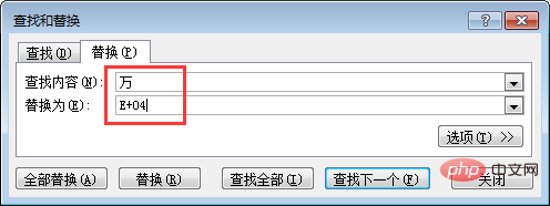
Select the data area, press the ctrl H shortcut key, in the dialog box, enter "Find content" and then " Thousands", enter "E 04" after "Replace with". "E 04" means 10 to the fourth power, which is ten thousand. This replacement turns the text data into data written in scientific notation.

Click "Replace All", you can see that the data containing "10,000" has become scientific notation data.

In the same way, replace "100 million" with "E 08", which means 10 to the 8th power, which is one hundred million.

After clicking "Replace All", the data becomes scientific notation data.

After selecting the data area, click AutoSum to sum the data.

Second method: Custom format method

If we want the data to be uniformly displayed at the "10,000" level after summation , then use customization as before.

After selecting the data area, press ctrl 1, click "Custom" in the pop-up dialog box, and enter the custom number format "0!.0,10,000" for "10,000" under "Type".

Then click "OK" to see the data results.

#The data displayed at this time is rounded off by default after the decimal point, leaving only one decimal place. If you want to see the original appearance of the data, you can see it in the edit bar.

Related learning recommendations: excel tutorial

The above is the detailed content of Practical Excel skills sharing: How to sum data with units?. For more information, please follow other related articles on the PHP Chinese website!