This article will take you through the OFFSET function, nicknamed the "King of Dynamic Statistics"! The OFFSET function is a very practical function. It plays an irreplaceable role in drop-down menus, dynamic charts, dynamic references and other operations. It is no exaggeration to say that a considerable part of the efficiency of Excel tables comes from OFFSET.

【Preface】
The OFFSET function is one of the important functions to determine whether Excel function users have advanced. In actual work, if you need to systematically and automatically model the data files at work, you will inevitably use this function.
[Function and Syntax]
The function of the OFFSET function is to use the specified reference as the reference system and return a new reference through the given offset.
Grammar: OFFSET(reference, rows, cols, [height], [width])

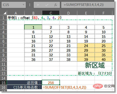


1. Basic general usage
As a regional reference for other functions, it should be the most basic use of the OFFSET function. The OFFSET function does not move the cell range, but returns an offset-expanded range address. Therefore, all functions that take a reference area as a parameter can use the return value of the OFFSET function, such as our example above Sum (OFFSET ()), or the following example:
2. Advanced general usage
Special skill ①: Simulate transpose TRANSPOSE function
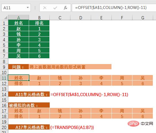
=OFFSET($A$1,COLUMN()-1,ROW()-11)
Transposing data is actually a process of "row to column" and "column to row". To be more specific, it is the issue of exchanging row numbers and column numbers. The "Name" column, the first column in the original data, becomes the first row in the new area after transposition. In the same way, the row number of each row in the "Name" column becomes the transposed column number. The principle of using OFFSET is to change the quotation range of the row and column numbers when taking the offset value.
★ For example, in cell A11, COLUMN()=1, 1-1=0, then the second parameter of OFFSET is 0, indicating that the number of rows of the original basic point is not offset (the second parameter of OFFSET indicates Row offset, if you are not familiar with it, please read the previous content!). ROW()=11, 11-11=0, the third parameter of OFFSET is 0, indicating that the number of columns is not offset, so the value of the original base point A1 cell is quoted.
★★ Pull the function to the right to fill, cell B11, COLUMN()=2, 2-1=1, then the second parameter of OFFSET is 1, indicating that the number of rows of the original basic point is downwards Move one position. ROW()=11, 11-11=0, and the third parameter of OFFSET is 0, indicating that the number of columns is not offset, so cell B11 refers to the value of cell A2 after the base point A1 is shifted downward.
★★★ Pull down the function of cell A11 to fill it. In cell A12, COLUMN()=1, 1-1=0, and the number of rows is not offset. ROW()=12, 12-11=1, the third parameter of OFFSET is 1, indicating that the column number is offset one position to the right from the basic point A1, and refers to the value of cell B1 (the reason why A1 in our formula is Use absolute references because all our cells are based on A1).
By analogy, when we use the mouse to pull down and right to fill in the formula, we use the COLUMN and ROW functions to help us locate the offset of each cell, thus achieving the transposition effect.
Stunt ②: Simulate the reverse query function of the Vlookup function

The reverse query of the VLOOKUP function is mostly completed with the help of arrays , but because of the array, the function may get stuck when there is a large amount of data, so many students will also use the INDEX function instead. So today, let’s enrich everyone’s knowledge. We use the OFFSET function to deal with this type of problem.
C12 cell function:
=OFFSET($A$1,MATCH("D2568",$B$2:$B$7,0),)
Function analysis:
We use cell A1 as the original base point, and the value that needs to be returned is in the same column as the original base point, so we only need to consider the row offset of the OFFSET function, no need to consider it Column offset. Because employee numbers are generally unique values, we use the MATCH function to get the serial number of the number "D2568" in the area B2:B7. The return value 4 is used as the row offset of the OFFSET function and is brought into the OFFSET function. =OFFSET($A$1,4,). If the column offset is omitted, the default is 0, and if the extended width and extended height are omitted, the default is 1 (that is, one cell). Isn’t it the A5 cell?
Stunt ③: Data reset upgraded version-rearrange data structure
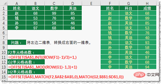
After entering the formula in the F2:H2 area, Pull down to fill in the data, and you will get the one-dimensional data table on the right. This kind of data rearrangement problem should be not uncommon in actual work! So what method will students choose to solve it? On the contrary, the author feels that the idea of the OFFSET function is more concise and clear.
Function analysis:
Step 1: Get consecutive names
F2 cell function:
=OFFSET($A$1 ,INT((ROW(F1)-1)/3) 1,)
Because there are three subjects in total, it can be determined that the same name needs to appear three times, then when we drop down cell F2 When filling the function, it is necessary to ensure that the parameter values of every three cells of the row offset of the OFFSET function are the same. Here we need to have a mathematical thinking of "divisor rounding". Let's list a picture to assist the explanation:

From the picture we can see a set of serial numbers, through INT((serial number-1)/3) After the conversion of 1, you can get the sequence on the right (if there are 4 subjects, change 3 to 4, and so on). Put this serial number into the second parameter of the OFFSET function as the standard for row offset, and you can get the effect of our name column.
Step 2: Assign different accounts to the same person
G2 cell function:
=OFFSET($A$1,,MOD(ROW(G1 )-1,3) 1)
Because each name in our column F appears three times, this determines that the three subjects of Chinese, mathematics, and English need to be listed sequentially and cyclically Come out, the same as the idea in the first step, use the mathematical thinking of "divisor and remainder" to achieve the effect.
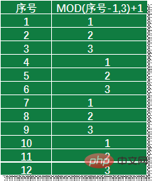
As shown in the figure above, the serial number is converted by the MOD function to obtain a sequential and cyclically listed serial number. Using this serial number as the third parameter column offset of the OFFSET function, the account content of the original data can be derived sequentially and cyclically.
The third step: simulate the INDEX function through the name and subject, and elicit the results from the original data
H2 cell function:
=OFFSET($A$1,MATCH(F2,$A$2:$A$5,0),MATCH(G2,$B$1:$D$1 ,0))
Use the MATCH function respectively to get the sequence number corresponding to the data in the relevant area, which is used as the offset of OFFSET and put into the second and third parameters respectively. The cell offset from the reference point A1 cell is the grade value we need.
Through the above content, we can easily find that the OFFSET function is often used in conjunction with the MATCH function. Because the Match function can find the sequence number of the keyword in an array, we often use this function to determine the offset of the OFFSET function.
3. Ideas for high-end applications
(Prototype of dynamic report template)
We use Excel for fast Geostatistically analyze data and quickly extract what we need. Now assume the following two scenarios:
Scenario 1:
The leader has arranged work to count the sales data of a certain quarter. We take action immediately and use functions to quickly create reports. ;
Scenario 2:
The leader arranged the work. Because sales data need to be collected every quarter, we have made the template in advance. As for when it will be given out Reports are up to us. Remember, don’t let “middle leaders” know that you are very productive.
Two scenarios, which approach would you choose? The author hopes it is the second one.
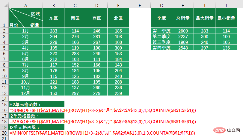
The idea determines the layout of our tabulation. This is a simple case. When the data source is modified, the corresponding quarterly data will be automatically adjusted. Not all positions in complex templates will use the OFFSET function, but for the need to dynamically reference data areas, it is absolutely correct to use the OFFSET function to handle it.
4. Typical usage examples
Stunt 4: Make a dynamic drop-down menu
In the data During the modeling process, we often use drop-down menus (or combo box controls). In order to ensure the uniqueness of the drop-down content, we will use the "Taiwan Balm" function of INDEX SMALL IF ROW to extract duplicate data from the array. Do you still remember the example where the OFFSET function replaced the INDEX function we talked about in the previous article? Therefore, if the OFFSET function can be used instead of the Index function, then the OFFSET function can also achieve the "one-size-fits-all" process. Let's take a look at the production process of a complex "drop-down menu".
Step 1: Use the OFFSET function to extract the unique value of the "Taiwan Balm" formula
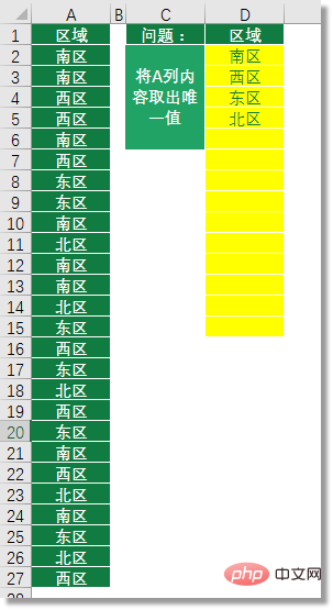
This formula is relatively long and is listed as follows:
D2 cell function:
=IFERROR(OFFSET($A$1,SMALL(IF(ROW($A$2:$A$27)-1=MATCH($A$2:$A $27,$A$2:$A$27,0),ROW($1:$20),9^9),<br>ROW(D1)),),"")
Tiger Balm Formula It's not the topic we want to talk about today, so I won't go into it. The important thing is to let everyone know that the OFFSET function can also achieve such a duplication effect.
Step 2: Use the OFFSET function in the name manager to establish a data source
We can use the Ctrl F3 key combination to open the name manager window, then create a new name and set the name to "Area ", the reference position is "D2:D15", as shown in the following figure:

Then select cell G1, press Alt D L key combination to open the data validation setting box, in Select "Sequence" in Allow, enter "=Area" in Source, as shown in the figure below:

Click the OK button, then the drop-down menu of our G1 cell will be created alright. But the problem also arises. We will find that there are many empty options, which is not what we need.

Some students will say that just select D2:D5 in the name manager. Yes, but if new data appears in the area of column A, there will be less data in the drop-down menu, so we still use the OFFSET function to deal with this problem at this time.
Change the reference position of "Area" in the name manager:

=OFFSET(Dynamic drop-down menu!$D$1,1, ,COUNTA(Dynamic drop-down menu!$D$2:$D$15)-COUNTBLANK(Dynamic drop-down menu!$D$2:$D$15),1)
Because the only value in our column D is obtained using a formula, the "empty cell" inside is not nominally "empty", but empty obtained by the formula, so it cannot be directly passed COUNTIF(D2:D15, "") to get the number of cells with values. Therefore, we first used the COUNTBLANK function (counting blank cells) to count the number of blank cells, then used the COUNTA function to count the number of non-blank cells, and finally subtracted the two to get the number of cells with values. . By using the obtained result as the fourth parameter of the OFFSET function (the number of expanded rows in the new area), the effect of dynamically referencing valid data is achieved. As shown in the figure below:
#If a new region name is added to column A, new options will also be added to the drop-down menu of G1. Let us take a look at the effect. , I believe this is what you need.
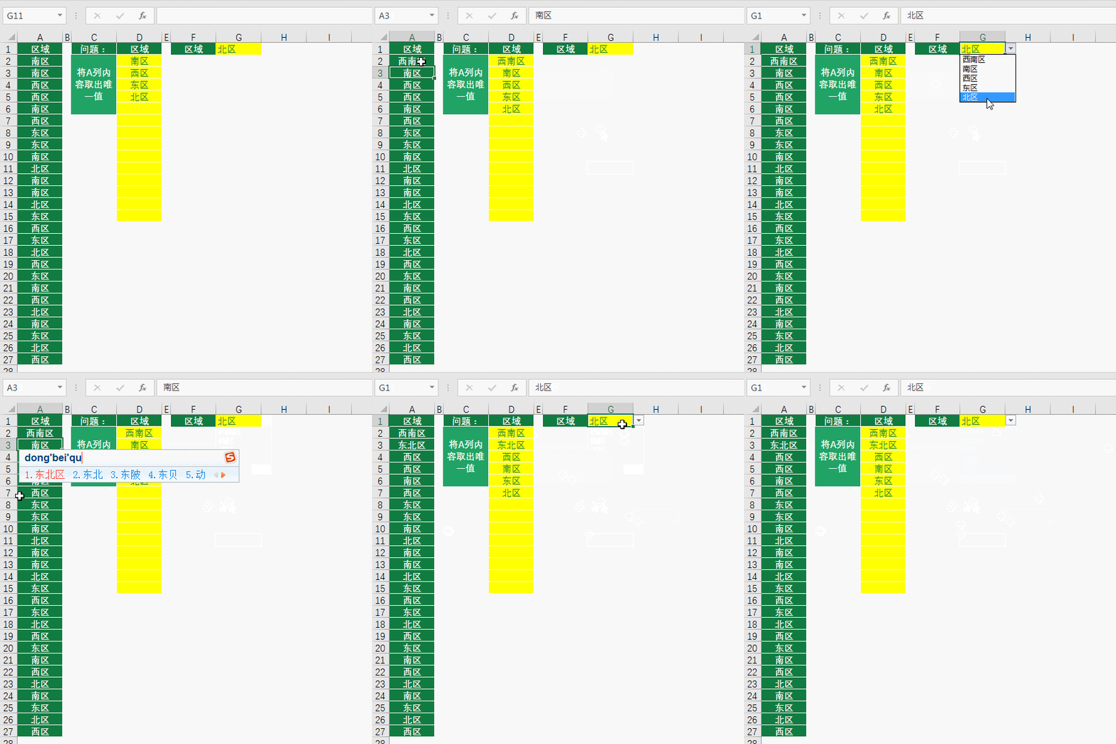
Stunt 5: Use of OFFSET function in charts
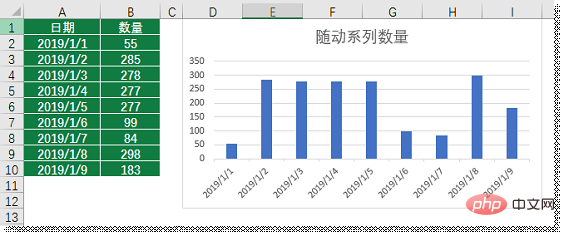
I believe everyone is familiar with the chart above. Strange. Students who are working will have experience in making charts. Select the area A1:B10 in the above picture, go to the toolbar - "Insert" - Column Chart to complete the content of our legend.
If we delete a row of data, there will be one less series legend in the column chart. However, if we add a row of data, we need to change the range of the chart data source to display the correct chart. But we can’t change it every time, otherwise we will lose the original intention of using Excel efficiently and quickly.
At this time, we can still learn from the OFFSET function to solve the problem:
Step 1: Use the OFFSET function to create custom names for the "date column" and "quantity column" respectively
Name manager, we have introduced it above, so I won’t say more. Select "Date Column" and set it as follows:
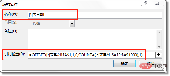
Reference position function:
=OFFSET(Chart Series!$A$1,1,0 ,COUNTA(chart series!$A$2:$A$1000),1)
Because there are no empty cells obtained by the formula in the original data, there is no need to use the Countblank function here, just use The CountA function counts the number of non-empty cells and can be used as the fourth parameter of the OFFSET function (the number of rows in the new area). A2:A1000 here represents an absolutely large area, ensuring that the newly input content is within this range.
Select "Quantity Column" and create a custom name for the quantity in the same way, as follows:
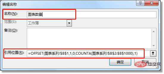
Step 2: Use the name
in the chart areaThis is the key to the OFFSET dynamic chart. The location where the name is added is very important.
In the drawing area, select any column, and in the edit bar you can see the function writing of the icon (is this the first time you know that charts also have functions). Let's modify the scope of the reference here.
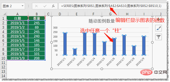
We only need to change the area.
Chart Series!$A$2:$A$10
Chart Series!$B$2:$B$10
Just replace these two red parts with custom names. Do not replace "Chart Series!$A$2:$A$10" as a whole!
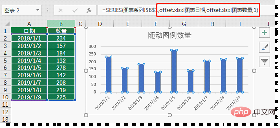
After replacing, press Enter, the function will be displayed as shown above, OFFSET.xlsx is the name of our workbook. The effect is as follows:
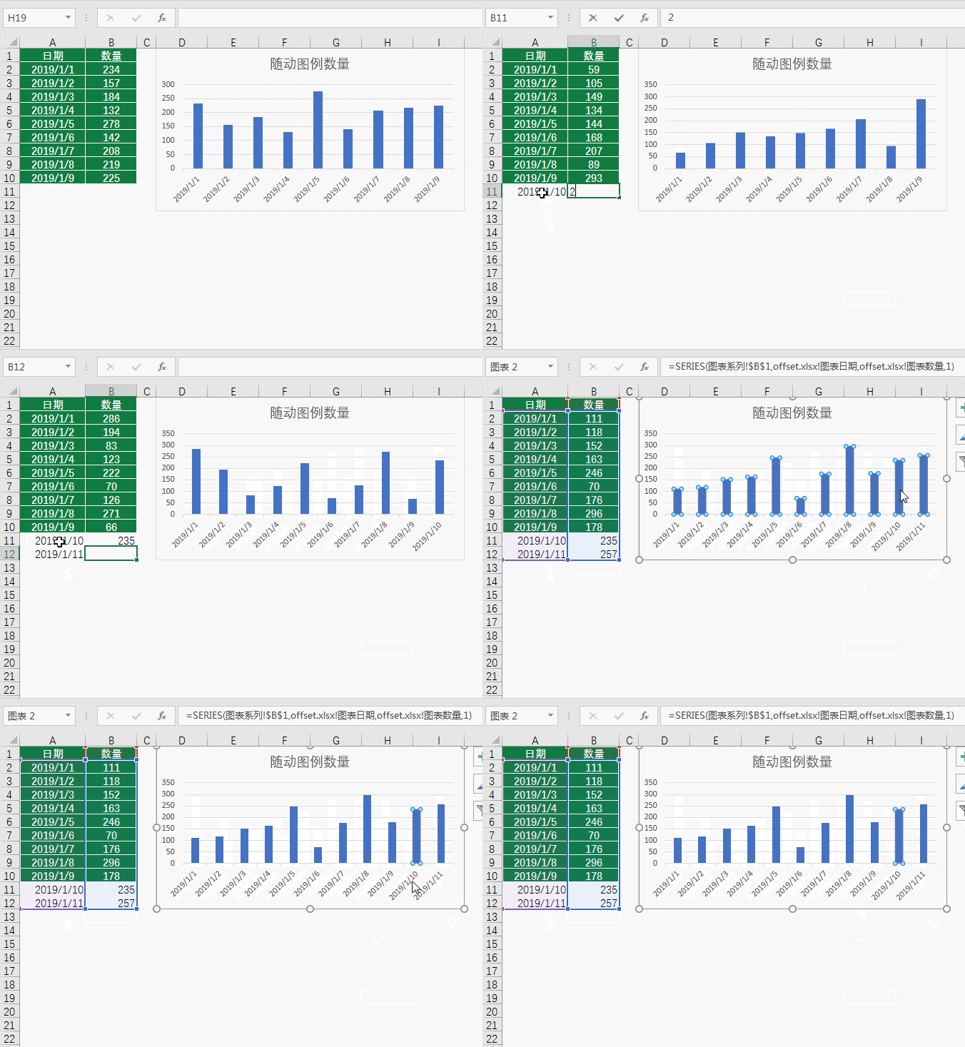
#Other chart types are also available. You can try to operate them to deepen your impression.
【Editor's Note】
The five parameters of the OFFSET function are not difficult to remember if you understand the meaning. Its return value can be used as a reference to other functions. Similarly, other functions whose "return value is in numerical format" can also be used as parameters of the OFFSET function, so that our data can move by itself.
This function plays an indispensable role in Excel functions. Especially when we need to use Excel modeling, this function is often used to reference dynamic areas and automatically process data. We strongly recommend that students We, if you can spend more time to learn, it will be of great benefit to your future watchmaking process.
Related learning recommendations: excel tutorial
The above is the detailed content of Excel function learning: Let's talk about the king of dynamic statistics OFFSET(). For more information, please follow other related articles on the PHP Chinese website!
 Compare the similarities and differences between two columns of data in excel
 excel duplicate item filter color
 How to copy an Excel table to make it the same size as the original
 Excel table slash divided into two
 Excel diagonal header is divided into two
 Absolute reference input method
 java export excel
 Excel input value is illegal


