The 4 most practical pivot table tips for learning Excel pivot tables

I didn’t learn much about functions, so I focused on pivot tables. Pivot tables don’t disappoint, there are always little things that can solve big statistical problems. The 4 home remedies here are just that.

The so-called folk remedies refer to prescriptions that are rarely seen in normal times but have special effects on specific situations. Today we share with you 4 "recipes" for pivot tables.

Recipe 1: Null value processing

When we perform data pivot on a set of data, we often encounter the situation where the corresponding data of a certain field in the value area is blank. . In the past, many partners made manual modifications. In fact, you can customize the blank display to 0 through a pivot table. (Note: Only for blanks in the value area!)

Example:

The purchase quantity of the screen 300*220 item in the first quarter is blank, and now the data needs to be pivoted and summarized.

After completing the pivot, we see that cell C13 is blank.

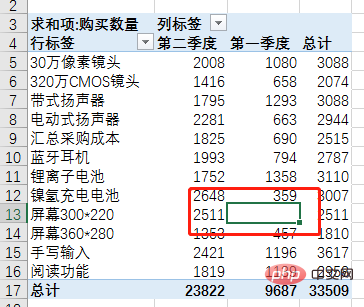
Click the PivotTable, right-click the mouse, and select [PivotTable Options].

Open the [Pivot Table Options] dialog box, check [Display for blank cells] in [Layout and Format], and at the same time, in the edit bar on the right Enter "No data" in the box.

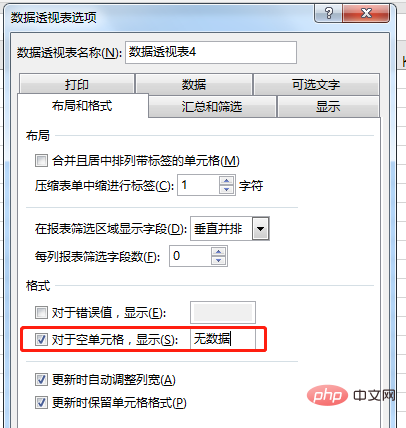
#After clicking OK, all the blank spaces in the PivotTable will be filled with "No Data" characters.

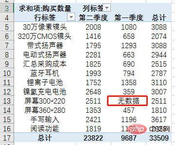
Note: Here we can fill the blanks with any text, numbers or symbols by definition.

Recipe 2: Ranking

In daily work, it is often necessary to rank the data after completing the data pivot. Many partners use the rank function to rank. In fact, pivot tables come with a ranking function, so there is no need for sorting or functions at all.

Still taking purchasing data as an example, now we have completed the data pivot.

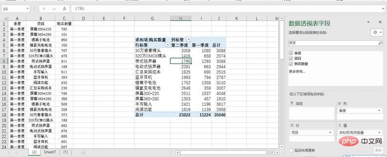
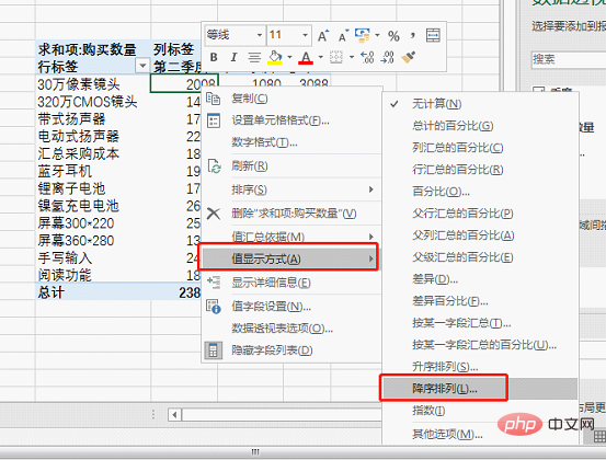
Select the pivot table, right-click the mouse, select [Value Display Mode], and select [Sort Descending] in the submenu.

Select items as the basic field for sorting and click [OK].

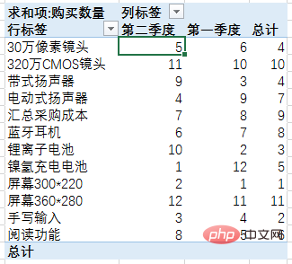
Finally we saw that the original purchase data information turned into ranking information.

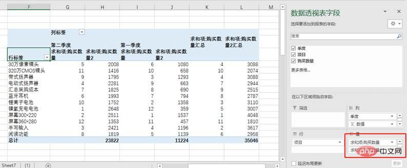
If we need to retain purchase data and ranking information at the same time, we only need to add the purchase quantity in the value field again.

Recipe Three: Create Worksheets in Batch

Batch creation is a task that is often encountered in daily life, such as creating branches, months , quarterly and other worksheets. If the number is small, we can create it one by one manually. What if the number is large? In fact, you can create worksheets in batches through pivot tables.

Example: Now we need to create a worksheet for 4 quarters.

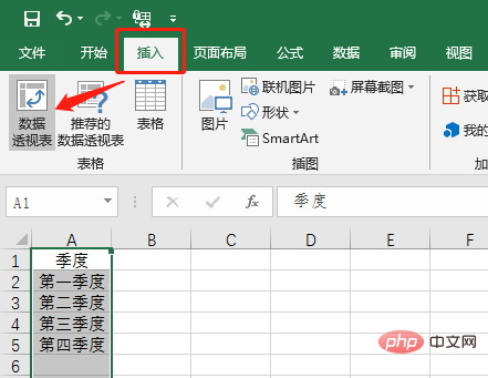
First enter the header quarter and the names of the four quarters in the table.

Then select the data in column A and click [Pivot Table] in the [Insert] tab.

In the [Create PivotTable] dialog box that opens, select the location of the PivotTable as an existing worksheet.

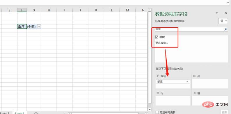
After confirmation, drag the [Quarter] field to the filter box.

Click the PivotTable, and then click [Options] - [Show Report Filter Page] in the [Analysis] tab.

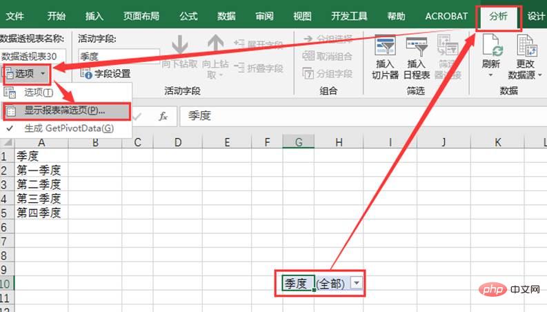
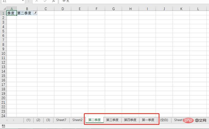
#The [Show Report Filter Page] dialog box appears, click OK directly, and we can see the batch-created worksheets.

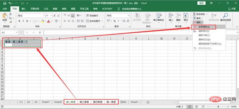
Select all the worksheets created, then select the unnecessary data in the table in any worksheet, and select "Start" - " Clear"-"Clear All" to complete the batch creation of worksheets.

Is not it simple?

Note: Worksheets created in batches are automatically sorted by worksheet name. For example, for the first to fourth quarters here, the created worksheets are second, third, fourth, and first quarter in order. If you want to create a worksheet in quarterly order, change the input to Arabic numerals, such as the 1st, 2nd, 3rd, 4th, etc. quarters. If you want to create worksheets in the order of the names you enter, an easy way is to add Arabic numerals 1, 2, 3, etc. in front of each name when inputting, and the worksheets will be created in the order of input.

Recipe 4: Group statistics by new fields

It is also a common thing to group data by new fields for statistics. For example, there are no months or quarters in the data, but your boss asks you to make statistics on a monthly or quarterly basis; there are no first-, second-, or third-class products in the data, but your boss asks you to make statistics on first-, second-, and third-class products. For this kind of statistics of original data according to newly specified fields, it can be very easily implemented using a pivot table.

Give two examples.

Example 1: Group statistics by date

The data source is sales registered by day. Now we want to count sales by month and quarter.

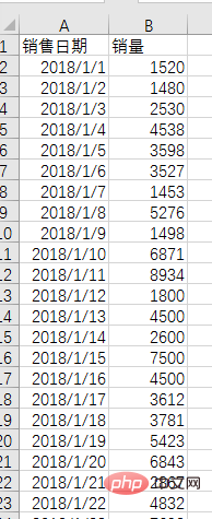
(1) Select all the data and insert the pivot table.

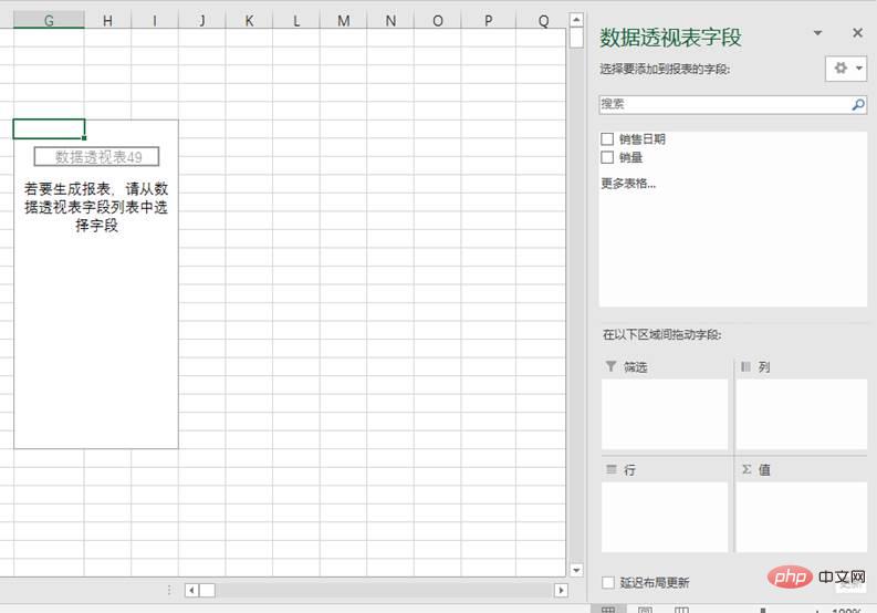
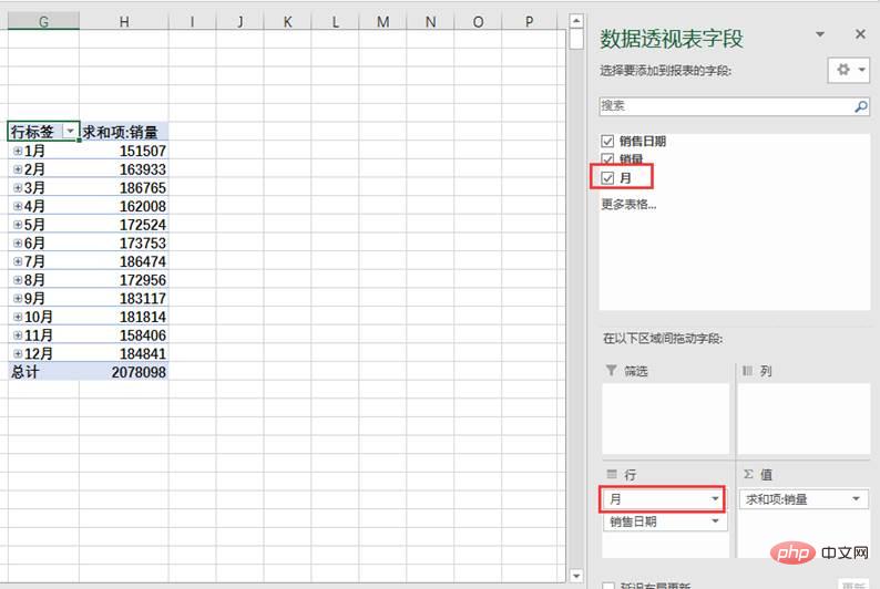
(2) Drag the "Sales Date" field into the row area, Excel will automatically add a "Month" field (requires the 2016 version), and the row in the right pivot table Tags are displayed by month. (Note: If you are using an earlier version, you need to set the "Quarter" field as shown below. Only after adding the "Month" field can statistics be calculated on a monthly basis.) Then drag "Sales" into the value area.

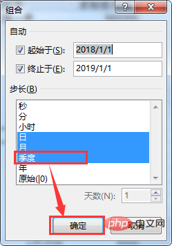
(3) Next we implement quarterly statistics through grouping settings. Right-click on any data under the pivot table row label and select the "Combine" command (you can also click [Analyze] - [Group Field] or [Group Selection]) to open the [Combine] dialog box. You can see that the two step sizes "day" and "month" have been selected.

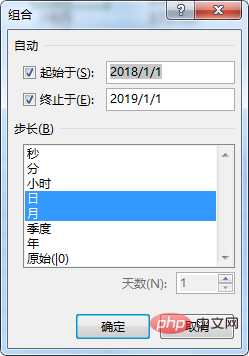
#Start at and end at data will be automatically generated based on the data source, don’t worry about it.

(4) Click "Quarter" and then OK.

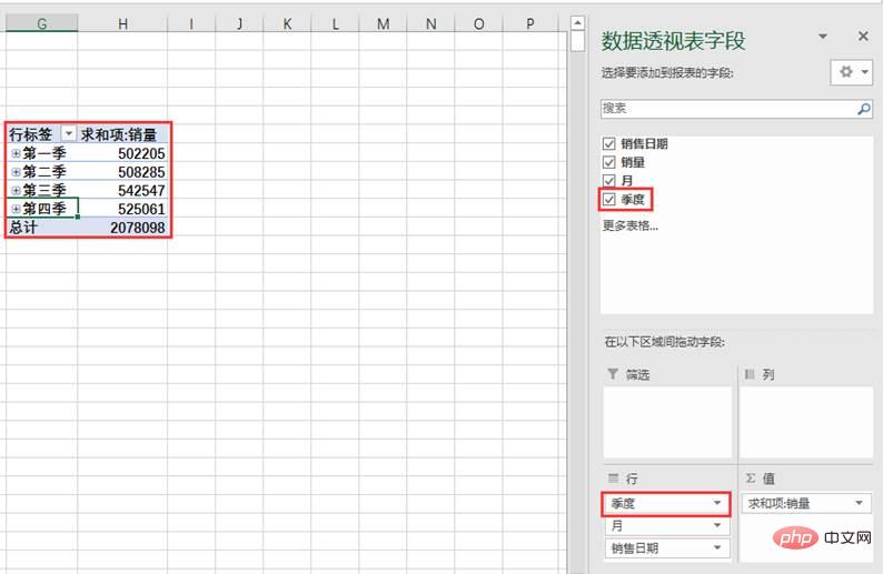
# (5) You can see that the "Quarter" field has been added to the pivot table field. In the pivot table on the left, click thesymbol to collapse the data and achieve quarterly statistics.

Example 2: Score statistics by stages

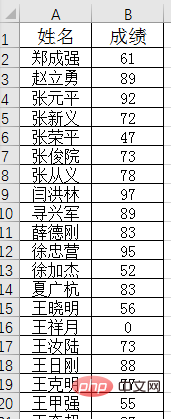
The following table shows the mathematics scores of a certain class, with only two fields: name and score. . Now we need to count the number of people in each stage, 60-79, 80-100.

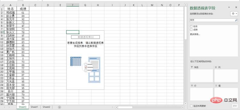
(1) Same as above, first create a pivot table.

(2) Drag the "Grade" field into the row area. At this time, a column of fractional values appears below the row labels of the left pivot table.

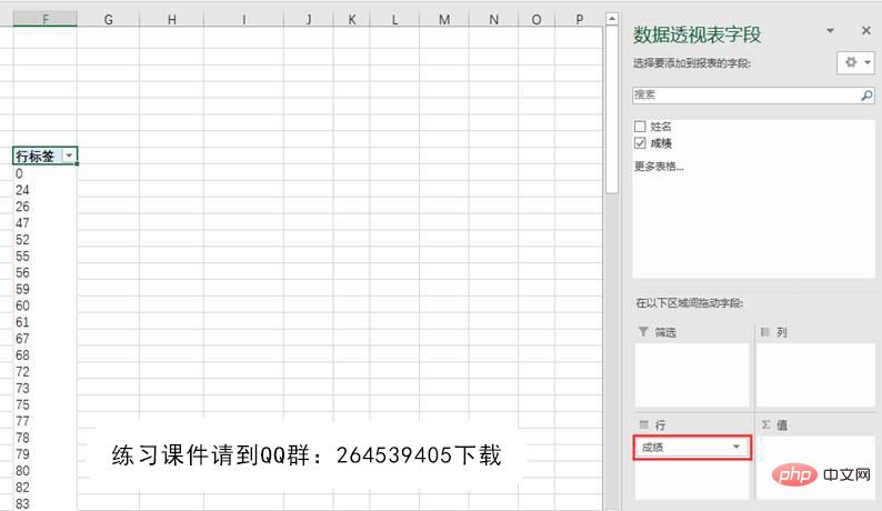
(3) Right-click on any score under the pivot table row label and select the "Combine" command to open the Combination dialog box.

# (4) Now modify the starting value, ending value, and step size as needed. The settings start at 60 and end at 100 in steps of 20, as follows.

(5) After clicking "OK", the row label changes to the three fractional segments we need.

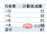
(6) Drag the "Grade" field to the value area to implement headcount statistics. For example, there are 11 people who failed.

(7) If you want to further see the names at each stage, you can drag the "Name" field into the row area.

If you want to segment more freely without being restricted by the step size, you can change the approach in step (3). For example, select 0-59, right-click, select "Combine", generate "Data Group 1", select "Data Group 1", enter "D" in the edit bar, change "Data Group 1" to "D", this It is the grade D stage; select 60-79, right-click the combination and change it to "C"; select 80-90, right-click the combination and change it to "B"; select 90 or above, right-click the combination and change it to "A". In this way, the results are divided into four stages ABCD for statistics.

Summary:

Today I shared with you 4 practical "recipes" for pivot table functions. These folk remedies are very efficient and can replace complex function work and improve efficiency. If you pay more attention to some functions and options in your daily work, and think more, you will find one more skill to make Excel run more freely.

Related learning recommendations:excel tutorial

The above is the detailed content of The 4 most practical pivot table tips for learning Excel pivot tables. For more information, please follow other related articles on the PHP Chinese website!