In the previous article "Sharing practical Excel skills: Making dynamic Gantt charts", we learned how to make dynamic Gantt charts in Excel. Today we are going to talk about Excel data drop-down menus and introduce how to make efficient search-style drop-down menus. Come and take a look!

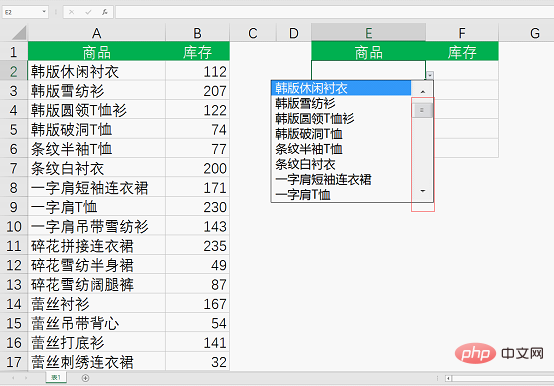
# At work, we often use Excel data validation to create drop-down menus to standardize data input and save data entry time. But when there are many data options in the drop-down menu, it will be difficult to find the data. For example, in the picture below, there are too many data options in the drop-down menu. It is time-consuming to "find" the required data items by dragging the scroll bar next to it, which directly reduces our work efficiency.

#So is there any way to solve this problem of too many options and hard to find data?
Yes, my method is the search drop-down menu!
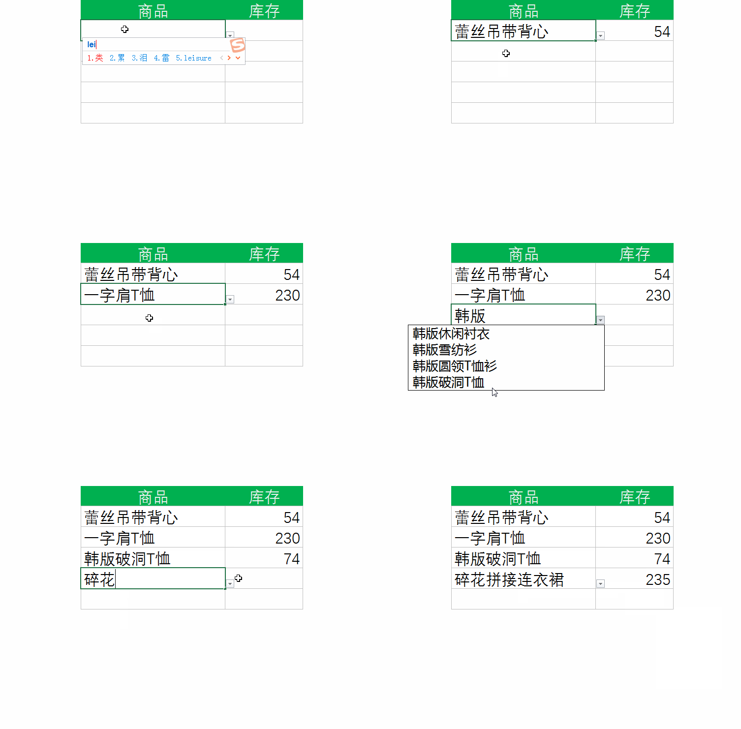
Just like searching on Baidu, after entering the keyword, a drop-down menu will pop up to display search questions containing the keyword for selection. The effect we want to achieve is to enter keywords in the cell, and then click the drop-down menu. Only the data containing the keywords will be displayed in the menu, thereby improving data entry efficiency.

The picture below is the data source for our tutorial. Note that the data source must be sorted by keyword, either in ascending or descending order.
Select the cell range E2:E6, click the [Data] tab, click [Data Verification], and select "Settings" in the pop-up "Data Verification" dialog box. Set the verification condition in the card to "sequence".
Enter the formula in the source:
=OFFSET($A$1,MATCH(E2&"*",$A$2:$A $17,0),0,COUNTIF($A$2:$A$17,E2&"*"),1)
OFFSET (reference frame, row offset, column offset, number of rows in the new reference area, number of columns in the new reference area)
As shown in the figure below, we need to select the cell range E2:E6 again and click the [Data] tab [Data Verification] button to enter the "Data Verification" dialog box and uncheck the "Error Warning" tab. [Show error warning when entering invalid data] option, and then click "OK".

Finally enter the formula =IFERROR(VLOOKUP(E2,$A$2:$B$17,2,0),"") in cell F2. Use the VLOOKUP function to find the location of the E2 value in the cell range A2-B17, and return the corresponding inventory in column 2 (that is, column B). 0 represents an accurate search. When an error value cannot be found and an error value is returned, use the IFERROR function to convert the error value to null.
At this point, the search drop-down menu is completed!
Search-style drop-down menus can exponentially improve data entry efficiency, especially when there are many drop-down menu options. Classmate, quickly open your excel and do some operations.

Related learning recommendations: excel tutorial
The above is the detailed content of Practical Excel skills sharing: making efficient search-style drop-down menus. For more information, please follow other related articles on the PHP Chinese website!
 Compare the similarities and differences between two columns of data in excel
 excel duplicate item filter color
 How to copy an Excel table to make it the same size as the original
 Excel table slash divided into two
 Excel diagonal header is divided into two
 Absolute reference input method
 java export excel
 Excel input value is illegal