Practical Excel skills sharing: four rating formulas

In the previous article "Sharing of Practical Excel Skills: Clever Use of [Ctrl] and [Shift] Shortcut Keys", we learned two commonly used Excel shortcut keys. Today we will talk about four ways to write rating formulas. I hope it will be helpful to everyone!

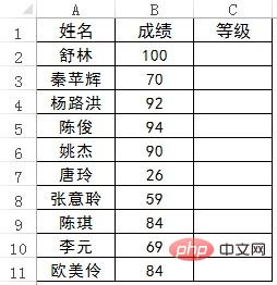
Teachers need to grade student performance. Results are expressed in the form of scores. How to automatically change the results to four levels: "fail, pass, good, and excellent".

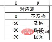
First create a level correspondence table in Excel, as follows:

Special reminder: the auxiliary correspondence constructed above The numbers in the table must be arranged from small to large. Reaching this score or exceeding this score is the corresponding level.

The first three formula writing methods below all take advantage of the approximate matching characteristics of the ascending order of the corresponding functions by arranging numbers from small to large. If the numbers are not arranged from smallest to largest, the result will be incorrect.

First, INDEX MATCH nesting

Enter the formula in cell C2:

=INDEX($ F$2:$F$5,MATCH(B2,$E$2:$E$5))

Second, VLOOKUP function

C2 cell input formula:

=VLOOKUP(B2,$E$2:$F$5,2)

VLOOKUP function is also often called The heartthrob function. Wherever there is a search, there is a VLOOKUP function.

I still remember that Teacher Tick Tak vividly told everyone how to use the VLOOKUP function in the Speedy Comprehensive Class. There are four parameters: the first is who to look for, the second is where to look, and the third is to return Which column is the value of, and whether the fourth parameter is to be found accurately or approximately.

In the case of this article, the fourth parameter of the VLOOKUP function is omitted, and the default is approximate matching. When searching, an exact match or an approximate match is returned. If an exact match is not found, the largest value less than the lookup value is returned.

Third, LOOKUP function

Enter the formula in cell C2:

=LOOKUP(B2,$ E$2:$F$5)

The first parameter of the LOOKUP function is the query value, and the second parameter is the query area. If the LOOKUP function cannot find the query value, it will match the largest value in the query range that is less than or equal to the query value.

Fourth, IF function

Enter the formula in cell C2:

=IF(B2

The IF function formula is the longest, but it can Write the formula directly without using the auxiliary correspondence table.

A question involves multiple functions and different ways of writing formulas. As Teacher Tick said, the better you master Excel functions, the more ideas and formulas you will have to solve problems. All roads lead to Rome, and approximate matching queries can be achieved with several functions. Use whichever one you like.

Related learning recommendations: excel tutorial

The above is the detailed content of Practical Excel skills sharing: four rating formulas. For more information, please follow other related articles on the PHP Chinese website!