How to display negative numbers in red brackets in Excel? In Excel, displaying negative numbers as red font within parentheses effectively highlights them. This tutorial is carefully written by PHP editor Xigua to help you easily implement this setting and make your data presentation clearer and more eye-catching.
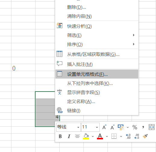
The operation method is as follows: 1. Open the Excel table on the computer, enter a set of data, then select the negative cell area, right-click the mouse, and select the [Format Cells] option in the drop-down menu that opens. .

The above is the detailed content of How to turn negative numbers entered in Excel into red brackets Tutorial on turning negative numbers into red brackets in Excel. For more information, please follow other related articles on the PHP Chinese website!


