Sharing practical Excel skills: Quickly sum data and add styles to subtotal rows

In the previous article "Practical Excel skills sharing: "Paste Special" turns out to have so many functions!》, we learned about the techniques of using Paste Special. Today we will talk about the processing skills of excel subtotal rows, and introduce how to quickly sum up data and add styles for multiple cross-row subtotal rows. I hope it will be helpful to everyone!

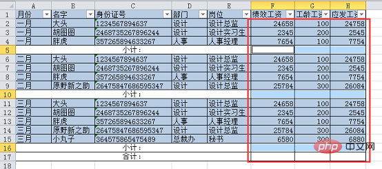
When you encounter multiple non-consecutive subtotal rows in the table,how do you sum them up?Here are two more convenient methods to introduce to you. The table is as follows:

Method 1:

Select the first summing area.

Click the "AutoSum" button drop-down menu under the "Formulas" tab and click Sum.

Follow this method, select each summing area below in turn, and sum it up. The final result is as follows:

You will find that this method is easy to handle when there are few "subtotal" rows, but it is very difficult when there are many "subtotal" rows. slow. Let me tell you a more concise method below.

Open your mind Method 2:

Drag the mouse to select the F2-H16 data area.

Press the "ctrl G" positioning shortcut key again to pop up the positioning dialog box. Click "Targeting."

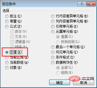
Select "Null Value" in the newly popped up dialog box, and click the OK button after setting it.

#At this point you will see that all empty cells are selected and appear light blue.

Click "Sum" in the drop-down menu of the "AutoSum" button under the "Formulas" tab, or directly press the sum shortcut "ALT =" . At this point all subtotal rows are automatically summed. The results are as follows:

#After completing the sum of the subtotal rows, we only need to select the "Total" row cell range.

Click "AutoSum" or press the shortcut key "Alt=", excel will automatically identify all subtotal rows, and sum the subtotal rows, and the final result as follows.

After completing the above summation,it is also very simple to set a unified and prominent cell stylefor all subtotal rows. Below I will tell you 3 ways to set the style of cross-row cells.

Method 1:

Select the A5-H5 data area.

Click the "Cell Style" drop-down menu under the "Home" tab and select any style.

#Then directly double-click the "Format Painter" button under the "Home" tab.

At this time, the format brush is locked and can be brushed multiple times continuously. Directly and continuously brush through the A10-H10 and A16-H17 areas, all subtotal rows and total rows will be set to the same style.

Click Format Painter again to cancel the lock state of Format Painter. The final result is as follows:

You will find that setting the style of cross-row cells in this way is very convenient when there is little data, but when there is a lot of data, even if you double-click the format painter, you still have to click on multiple row numbers to set all the subtotal row cells. Grid style. Let me show you a more concise method.

Method 2:

Select the entire table area.

Click the "Filter Button" under the "Data" tab to set the filter drop-down menu button for the table.

#After setting the filter, a drop-down button will appear in each cell in the first row of the table.

Click the drop-down menu of "Month", check "Subtotal" and "Total", and click the OK button after setting.

At this point we can see that there are only subtotal rows and total rows in the table, and other rows are hidden.

Select the area A5-H5.

Press the shortcut key "ctrl shift down arrow key" to quickly select a continuous area. At this time, no matter how many subtotal rows there are below, they will be selected together.

Click the "Cell Style" drop-down menu under the "Home" tab, select any style to see the results.

Check "Select All" in the "Month" drop-down menu, and click OK after setting.

At this time, the hidden rows will be displayed, and the entire worksheet can be seen.

Three ways to open your mind:

We were doing the sum of subtotal rows earlier At the time, the method of positioning the null value was used. In fact, this method can also be used to set the style here. You may have questions here. As shown in the figure below, the first cells of the subtotal row and total row are merged cells and have characters. Can they be selected by positioning null values?

Let’s give it a try. Follow the previous operation method, select the entire table area, press the positioning shortcut key "ctrl G", check "Null Value", and click OK. We can see the following results:

You will be surprised to find that both the subtotal row and the total row here are selected and highlighted in blue. (The A5-E5 cells here are also selected, because they are the first cell among all the selected empty cells. They are in the editing state by default, so they are white)

The reason is:When we merge and center several cells, the cell saves the content and address of the upper left corner cell by default.This means that in the above picture, only the first cell of the subtotal row and total row has content, and cells B-E are empty values, so when we position the empty values, cells B-E will be selected, and they It is merged with the cells in column A, so they will be selected together.

It’s very simple at this point. We directly click “Cell Style” under the “Home” tab, select any style, and complete the setting. The results are as follows:

#Do you think it’s amazing? When we start to delve into Excel, we will find that we fall in love with this software, and our work will become more interesting!

Related learning recommendations:excel tutorial

The above is the detailed content of Sharing practical Excel skills: Quickly sum data and add styles to subtotal rows. For more information, please follow other related articles on the PHP Chinese website!