Excel pivot table learning value field settings

In the previous article "Practical Excel Tips Sharing: Using Pivot Tables to Summarize Performance", we learned about Excel Pivot Tables and how to use Pivot Tables to summarize performance. Today we continue to learn Excel pivot tables and talk about value field settings. I hope it will be helpful to everyone!

At the end of the previous pivot table tutorial, I leave a small question for my partners: How to adjust the implementation department according to the first, second and third departments of the pivot table on the left below? Partially sorted, the effect is as shown on the right.

There is no pivot table sorting here. Drag the cells directly in the pivot table to change the arrangement of departments. Please watch the picture below for the animation operation:

Today is the second section of our pivot table tutorial: value field settings.

1. Where is the value field set?

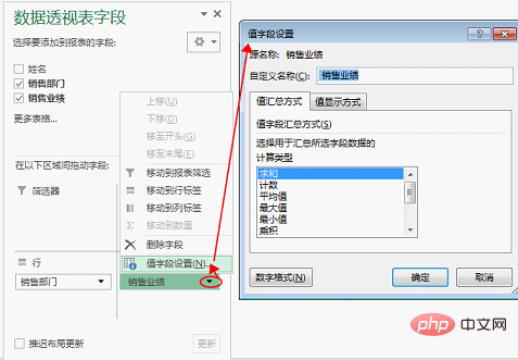
In the pivot table---right-click---display the field list, the "Pivot Table Fields" dialog box appears. Click "Values" and then select "Sales Performance" - select "Value Field Settings".

#2. What is the function of value field setting?

Change the value summary method, such as sum, count, maximum value, average value, minimum value, etc.

The pivot table defaults to summation. We can implement counting and other summary methods through settings.

3. Case demonstration value field setting operation

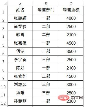
The following is the sales performance data table of each department:

Through the pivot table, use the value field settings to quickly calculate three questions:

• Sales performance summary of each department

• What is the highest performance of each department

• What is the lowest performance of each department

The pivot table statistical results are as follows:

The following is a demonstration of the operation steps:

Related learning recommendations:excel tutorial

The above is the detailed content of Excel pivot table learning value field settings. For more information, please follow other related articles on the PHP Chinese website!