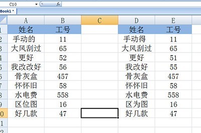
Take the following table as an example. The left side is the original data, and the right side is the data to be checked. To the naked eye, the two tables are somewhat similar.

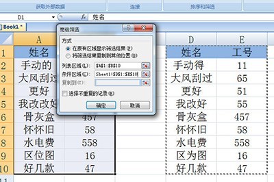
First select the original data on the left, and then click [Advanced] in [Data]-[Filter]. In the condition area, select the table to be checked on the right.

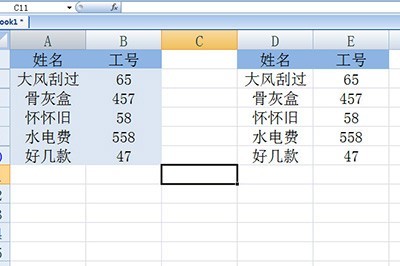
After clicking OK, the data will be filtered out, and then fill the original data table on the left with a color.

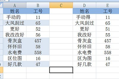
Finally click [Clear] in [Data]-[Filter], all the data will be restored, and then the data without color in the left table is the wrong data, please Check it carefully.

The above is the detailed content of Basic method of checking name and job number in Excel. For more information, please follow other related articles on the PHP Chinese website!


