How to add drop-down menus to dynamic charts in Excel

php editor Xigua will share with you how to add a drop-down menu in Excel today. By adding drop-down menus in Excel, the accuracy and efficiency of data entry can be greatly improved. When processing large amounts of data, drop-down menus can reduce input errors and save time. They are a very practical function in Excel. Next, let us learn how to add a drop-down menu in Excel!

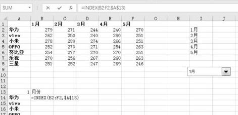
1. Use month as the filtering condition to observe the monthly sales of major mobile phone brands. In the blank area of ​​Excel, enter January to May vertically.

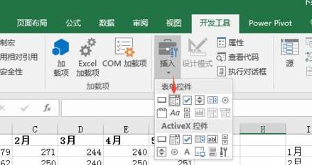
2. Insert the drop-down control, development tools--insert--form control--combo box, and pull out a drop-down box in the blank area of ​​the table.

3. Right-click the drop-down box control, select Set Space Format--Control, and set it as shown in the picture. A13 is a blank cell.

4. As shown in the picture, start inputting the major mobile phone brands at the position of A14. Enter the formula =INDEX(B2:F2,$A$13) at the position of B14. Pull down, A13 When the pull-down position is January, it is 1, and when it is pulled down to March, it is 3.

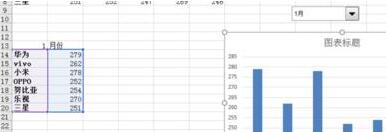
5. Select the data in the chart, insert the histogram, then place the drop-down control in the upper right corner of the chart, select the chart, and place it at the bottom.

6. Delete the vertical axis and horizontal line in the chart, and then adjust the color of each mobile phone brand.

The above is the detailed content of How to add drop-down menus to dynamic charts in Excel. For more information, please follow other related articles on the PHP Chinese website!