How to calculate the average of a set of cells in Microsoft Excel

Suppose you have a set of numbers and you need to find their average. It could be anything, it could be the score on your student roster, it could be the number of visits to your website per month. It's completely impossible to manually calculate the average and populate it into an Excel column. If we have a perfect solution that automates the entire process, you don’t need to prioritize manual operations.

Keep reading to learn how to easily find the average of a group of cells in an Excel worksheet using a quick formula and populate the average of an entire column with a few simple clicks.

Solution

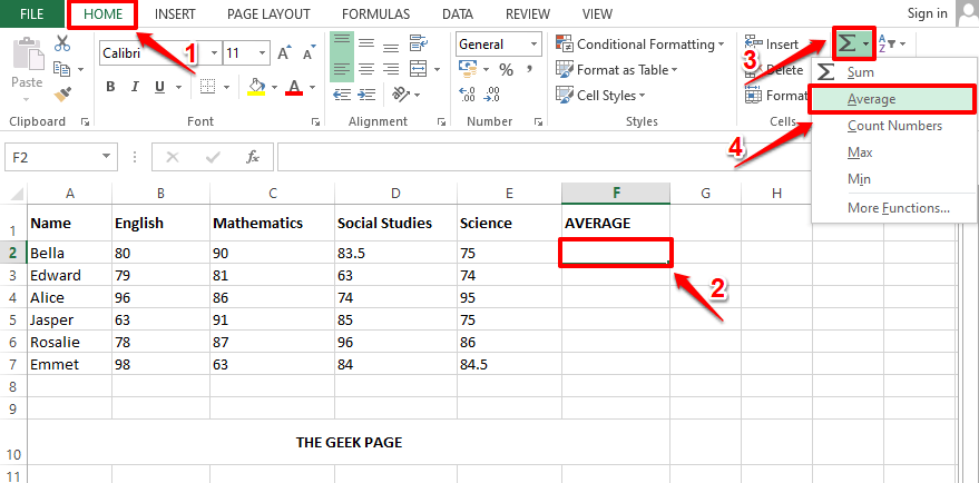
Step 1: Suppose you have a column named AVERAGE whose value needs to be calculated with each student Fill in the corresponding average of the values ​​present in each row.

To do this, first click the first cell of the AVERAGE column .

Then make sure you are in the HOME tab at the top. Next, click the drop-down menu associated with the Sigma button and select Average from the list of options.

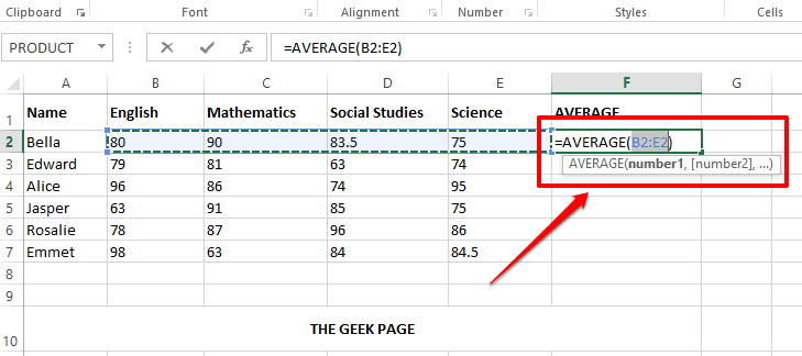
Step 2: All values ​​appearing in the row of the selected cell will be automatically considered to calculate the average. In the example screenshot below, the average function auto-populates as =AVERAGE(B2:E2). Here B2:E2 represents all the cells from B2 to E2 in the Excel worksheet.

NOTE: If you need to make any changes, you can always edit the parameter list inside the AVERAGE() function. Suppose if you only need to find the average of cells C3 and D3, then your Average() function would be =AVERAGE(C3, D3). You can also provide static values ​​as parameters in the Average() function. For example, your Average() function could also be =Average(4,87,34,1).

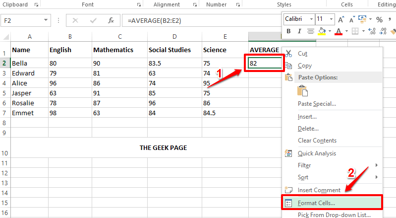
Step 3: Now if you press the Enter key, you can see that the average is calculated successfully. But the decimal point may not be present. If this is the case, right-click the cell and select "Format Cell " from the right-click context menu option.

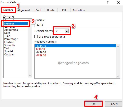
Step 4: In the Set CellsFormat window, make sure you are in step atab.

Now, under the Category option, click on Number.

To the right of , enter the number of decimal places you want in the decimal placesfiller. I gave 2 in the screenshot below.

Click the OK button after completion.

Step 5: You are here! Average values ​​now also have decimal places visible. If you want to apply the same formula to the rest of the cells in the same column, just click and drag down the little square icon in the lower right corner of the formatted cell.

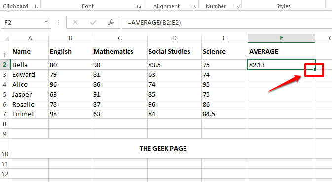
That’s it. Your formula to find the average of a group of cells is now successfully applied to all cells present in the same column.

The above is the detailed content of How to calculate the average of a set of cells in Microsoft Excel. For more information, please follow other related articles on the PHP Chinese website!