
When you have a lot of data, it often becomes increasingly difficult to analyze it. But does it really have to be this way? Microsoft Excel offers an amazing built-in feature called Pivot Tables that can be used to easily analyze huge chunks of data. They can be used to efficiently aggregate your data by creating your own custom reports. They can be used to automatically calculate the sum of a column, filters can be applied to it, the data within it can be sorted, etc. The things you can do with pivot tables and how to use them to ease your daily excel hurdles are endless.
Keep reading to learn how to easily create a Pivot Table and learn how to organize it effectively. Hope you enjoyed reading this article.
In very basic terms, you can think of a PivotTable as a dynamic report. However, there is a huge difference between reports and pivot tables. Reports are static, they do not provide any interaction. But unlike them, PivotTables allow you to view your data in many different ways. Additionally, a PivotTable does not require any formulas to form the data it holds. You can apply many filters on the pivot table and customize the data as per your requirements.
In this article, we created a sample table that contains data for creating a PivotTable report. In the example table we created, there are columns Date, Item, Units Sold, and Profit. We are mainly interested in finding the daily total profit based on different projects. Let's see how to do this with detailed steps and examples.
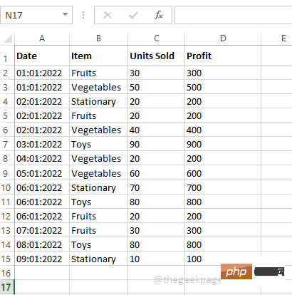
Creating a Pivot Table is very easy once you have your data ready.
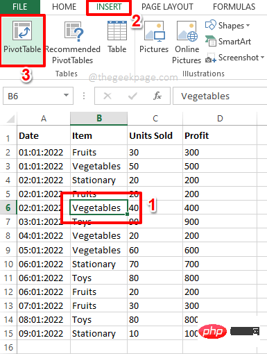
Step 1: Click anywhere within the data. Next, click the Insert tab on the top ribbon. Now, click on the button named Pivot Table.
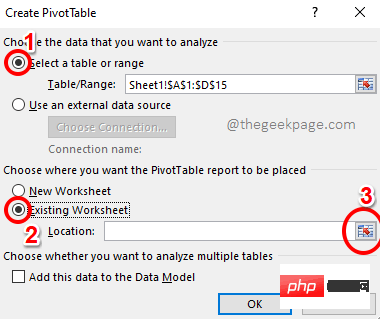
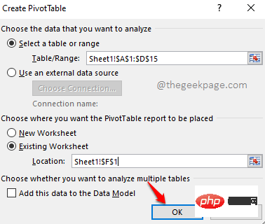
Step 2: NowCreate PivotDataTable window launches in front of you.
Under the "Select data to analyze" section, the radio option corresponding to the "Select a table or range" option will be selected by default Button. If there is no selection, select it.
Now, under the Select where you want the PivotTable to be placed section, you can choose to place it in a New worksheet or Existing worksheet Create a pivot table in the table.
If you select New Worksheet, the PivotTable will be created in a different worksheet. However, it is easier to compare the PivotTable and our sample data if they are both on the same worksheet, so I selected the Existing Worksheet option.
After selecting the radio button corresponding to the existing worksheet, click Select Cell# on the position field ## button.
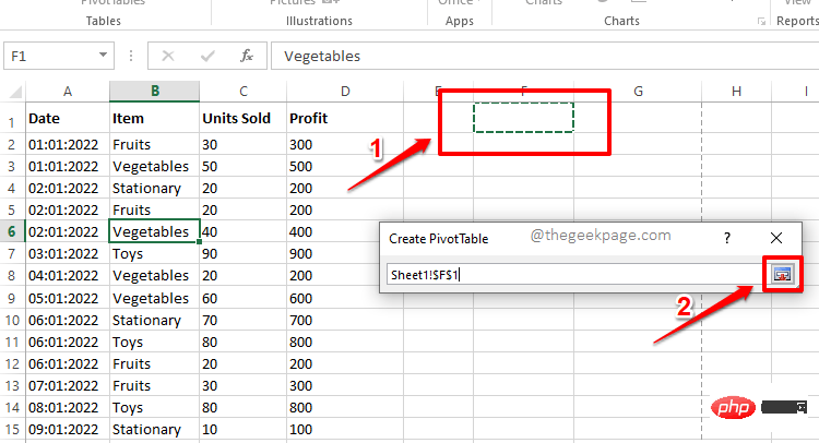
Step 3:Create PivotDataThe table window will now be minimized. Click the cell where you want to start the PivotTable report. After selecting the cells, click the "Select Cells" button again to maximize the window.
Step 4: After returning to the "Create PivotTableTable" window, click "OK" button.
Step 5: That’s it. Your PivotTable report is now inserted into your worksheet. In the following sections, let us see how data is generated in a PivotTable and how to manipulate the data.
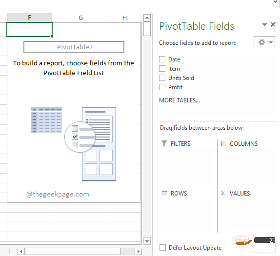
Step 1: Suppose you want to see the sum of profits . You don't need to write any formulas for this.
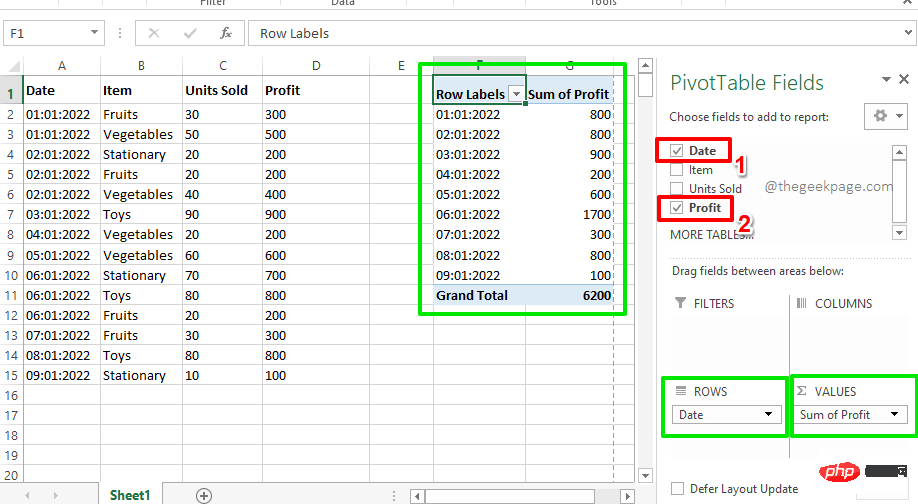
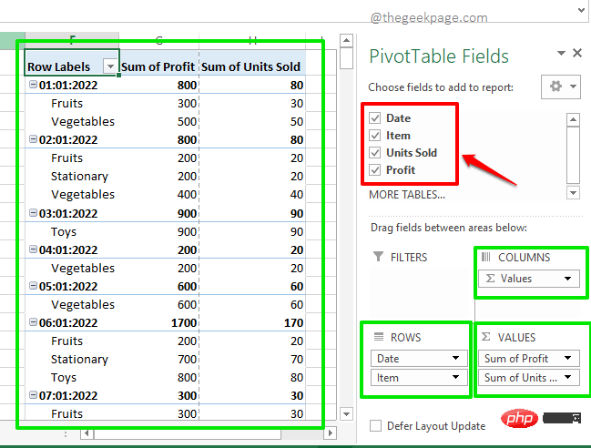
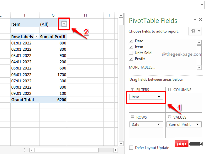
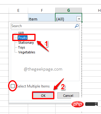
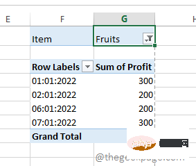
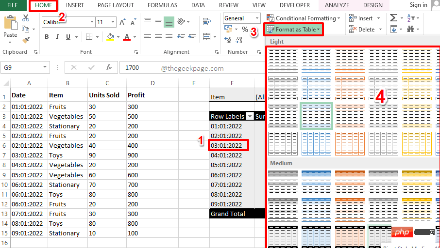
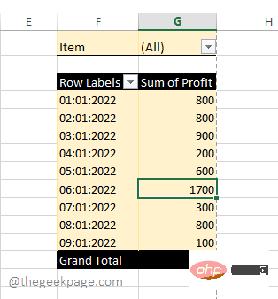
In theright pane where the Pivot table settings are located, you simply click on the # corresponding to the Profit column ## Checkbox. If you look at your Excel worksheet, you will see that your PivotTable now only has one column and it reads Sum of Profit. It calculates the sum of all available profits in the sample data. Step 2: Now let’s say you want to see the total profit, but at the same time, you also want to see the daily profit. In this case, also select the checkbox corresponding to the Date column in the right pane. Now, the Date column will automatically be located below the ROWS section of the PivotTable and your PivotTable will successfully display the profit for each day. Finally, it also shows the total of the profit earned. Step 3: Now, let us try to select the checkboxes corresponding to all the columns in the sample data. Well, this provides a perfect report in your pivot table showing the profit per project per day. Well, it couldn’t be more organized and we agree! If you only want to view the PivotTable after applying some specific filters , there are also some ways to do this. For example, if you want to view the daily profit of only the fruit project, you can follow the steps below. Step 1: First, on the right side of the window , drag the Item field from PivotTable Fields Put it in the FILTERS section. This simply adds filter items to your pivot table. Now on the PivotTable you will see the newly added filter Item. Click the drop-down menu associated with it. Step 2: Now click on the item Fruits and click on the OK button to filter only Pivot table of Fruits. Note: You can also choose to apply multiple filters on the PivotTable. You can do this by enabling the Select multiple items checkbox that corresponds to the circle marked in the screenshot below, then selecting multiple fields Step 3: If you look at the pivot table now, you can see that each day consists of only Fruits itemsTotal profit obtained Step 1: First click Now, make sure you are on the "Home" tab. Next, click the drop-down Format as Table. From the list of available styles, select any style Step 2 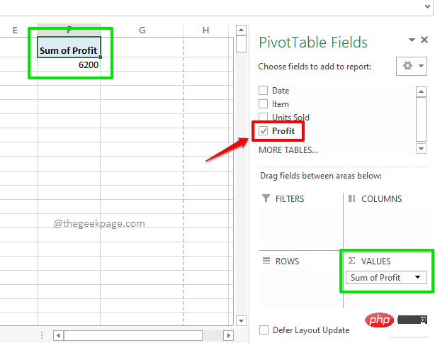
Part 5: How to Apply Filters in PivotTable
The above is the detailed content of How to create a PivotTable in Microsoft Excel. For more information, please follow other related articles on the PHP Chinese website!
 What are the four big data analysis tools?
 How to clear the WPS cloud document space when it is full?
 How to run phpstudy project
 Where does the subscript of php array start?
 Website creation software
 What is the difference between golang and python
 Why is there no response when headphones are plugged into the computer?
 How to operate Oracle rounding


