Numerical distance based on machine learning: the distance between points in space

This article is reproduced from the WeChat public account "Living in the Information Age". The author lives in the information age. To reprint this article, please contact the Living in the Information Age public account.

In machine learning, a basic concept is how to judge the difference between two samples, so as to be able to evaluate the similarity and category information between the two samples. The measure to judge this similarity is the distance between two samples in the feature space.

There are many measurement methods based on different data characteristics. Generally speaking, for two data samples x, y, define a function d(x, y). If it is defined as the distance between the two samples, then d(x, y) needs to satisfy the following basic properties ：

• Non-negativity: d(x,y)>=0
• Identity: d(x,y)=0 ⇔ x=y
• Symmetry: d (x, y) = d (y, x)
• Triangle inequality: d (x, y)

Generally speaking, common distance measures include: distance between points in space, distance between strings, similarity of sets, and distance between variable/concept distributions.

Today we will first introduce the distance between the most commonly used points in space.

The distance between points in space includes the following types:

1. Euclidean Distance

There is no doubt that, Euclidean distance is the distance that people are most familiar with. It is the straight-line distance between two points. Students who have studied junior high school mathematics all know how to calculate the distance between two points in two-dimensional space in the Cartesian coordinate system

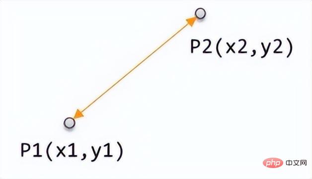
The calculation formula is:

##The Euclidean distance extended to N-dimensional space is:

2. Manhattan Distance

Manhattan distance is also called taxi distance. Its concept comes from the many horizontal and vertical blocks in Manhattan, New York. , in this kind of neighborhood, if a taxi driver wants to walk from one point to another, it is useless to calculate the straight-line distance, because the taxi cannot fly over the buildings. Therefore, this distance is usually calculated by subtracting and adding the east-west and north-south distances of two points respectively. This is the actual distance that the taxi has to travel.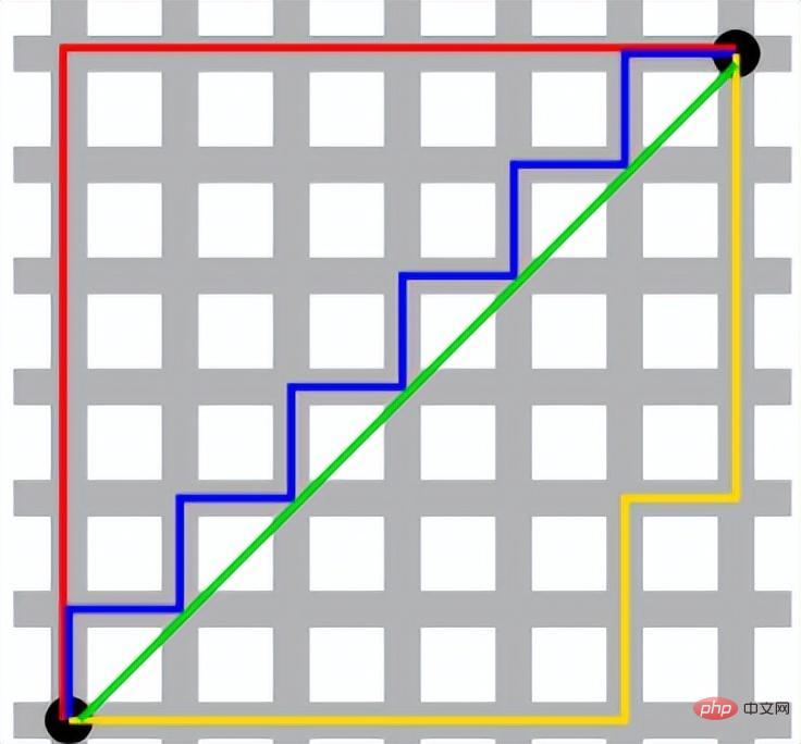

As shown in the figure, the red line and the yellow line are the Manhattan distances of two different paths. Mathematically, the calculation method of Manhattan distance in two-dimensional space is as follows:

3. Chebyshev Distance (Chebyshev Distance)

Chebyshev distance is defined as the maximum value of the difference in coordinate values ​​between two points.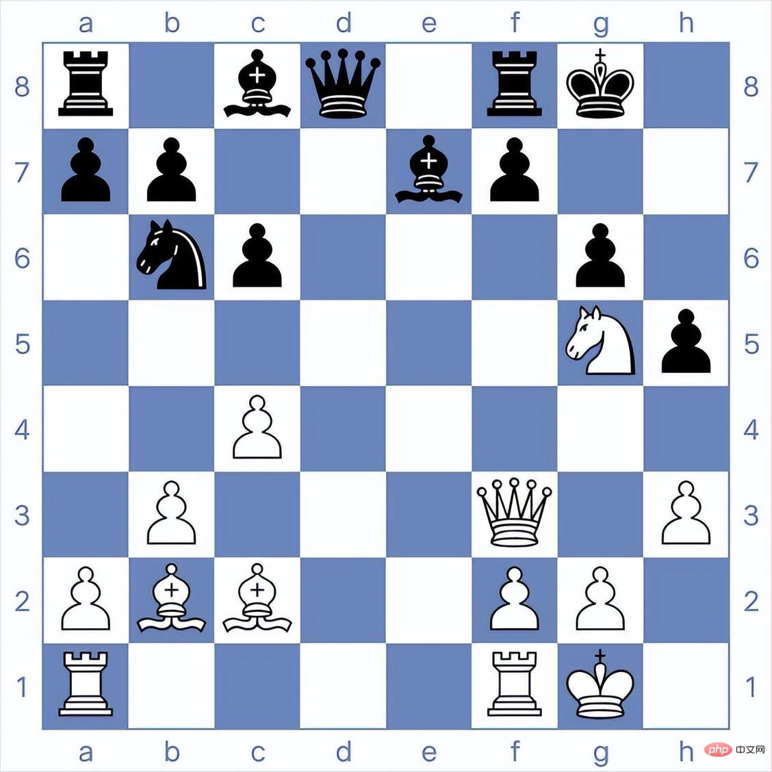

The most intuitive example is the king in chess, because it can move sideways, straight, and diagonally, but it can only move one square at a time, so it can move The Bishev distance is the minimum distance required to move to another square.

##4. Minkowski Distance

The Min distance itself is not a special distance, but a formula that combines multiple distances (Manhattan distance, Euclidean distance, Chebyshev distance).

It is defined as, for two n-dimensional variables, the Min's distance is:

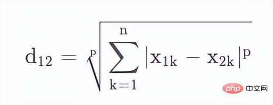
When p=1, you can see

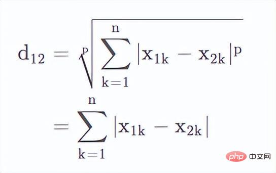
At this time is the Manhattan distance.

When p=2, you can see that

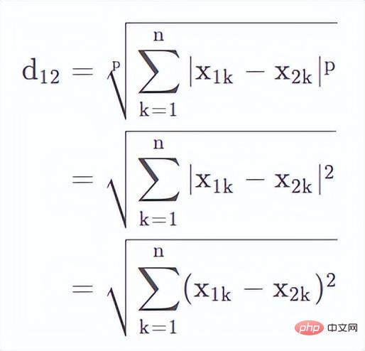
is the Euclidean distance.

When p=∞, you can see that

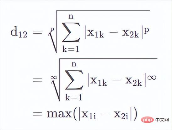
This is the Chebyshev distance.

5. Standardized Euclidean Distance

Euclidean distance can measure the straight-line distance between two points, but in some cases In some cases, it may be affected by different units. For example, if there is a height difference of 5 mm and a weight difference of 5 kg at the same time, the perception may be completely different. If we want to cluster three models, their respective attributes are as follows:

A: 65000000 mg (ie 65 kg), 1.74 m

B: 60000000 mg (ie 60 kg) , 1.70 meters

C: 65,000,000 mg (i.e. 65 kg), 1.40 meters

According to our normal understanding, A and B are models with better figures and should be classified into the same category. However, when actually calculating in the above units, it is found that the difference between A and B is greater than the difference between A and C. The reason is that the different measurement units of attributes lead to excessive numerical differences. If the same data is changed to another unit.

A: 65kg, 174cm

B: 60kg, 170cm

C: 65kg, 140cm

Then we will get The result that comes to mind is that A and B are classified into the same category. Therefore, in order to avoid such differences due to different measurement units, we need to introduce standardized Euclidean distance. In this distance calculation, each component is normalized to an interval with equal mean and variance.

Assume that the mean (mean) of the sample set X is m and the standard deviation (standard deviation) is s, then the "standardized variable" of X is expressed as:

##Among them, the standardized value = (the value before normalization - the mean of the component) / the standard deviation of the component. After simple derivation, we can get the standardized Euclidean distance formula between two n-dimensional vectors as:

If the reciprocal of the variance is regarded as A weight, this formula can be regarded as a weighted Euclidean distance. Through this operation, we effectively eliminate the differences between different weight units.

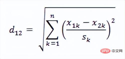
6. Lance and Williams Distance

Lance distance is also called Canberra distance,

It is a dimensionless indicator, which overcomes the shortcomings of Min's distance related to the dimension of each indicator, and is not sensitive to large singular values, and is especially suitable for data with scheduling bias. But this distance also does not take into account the correlation between variables. Therefore, if you need to consider the correlation between variables, you still need Mahalanobis distance.

7. Mahalanobis Distance

After standardizing the values, will there be no problems? maybe. For example, in a one-dimensional example, if there are two classes, one class has a mean of 0 and a variance of 0.1, and the other class has a mean of 5 and a variance of 5. So if a point with a value of 2 should belong to which category? We intuitively think that it must be the second category, because the first category is obviously unlikely to reach 2 numerically. But in fact, if calculated from the distance, the number 2 must belong to the first category.

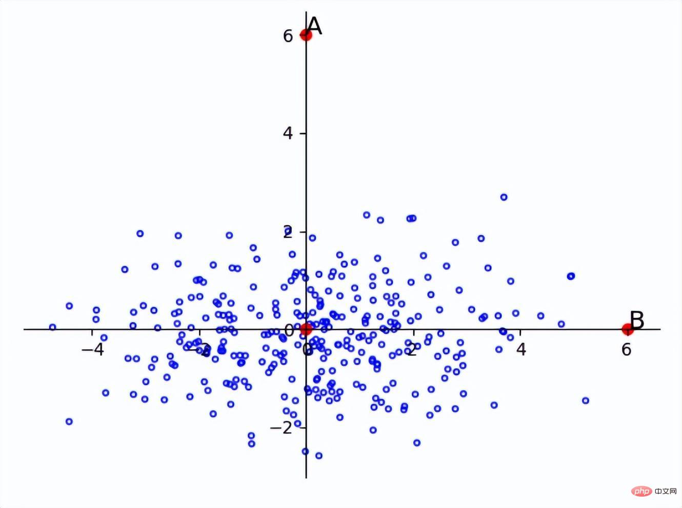
So, in a dimension with small variance, a small difference may become an outlier. For example, in the figure below, A and B are at the same distance from the origin, but since the entire sample is distributed along the horizontal axis, point B is more likely to be a point in the sample, while point A is more likely to be an outlier. .

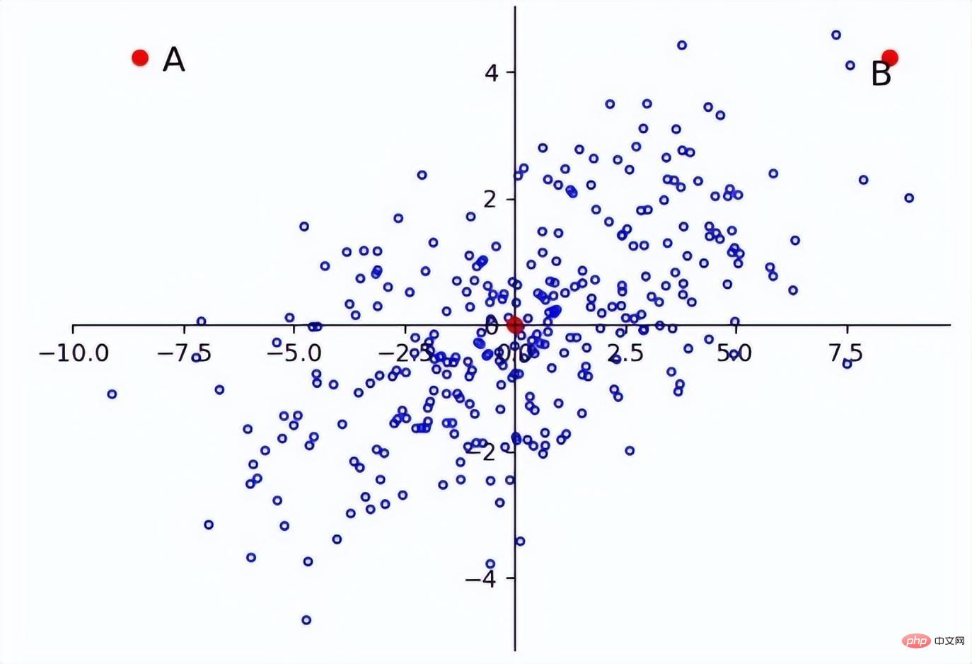
Problems may also occur when the dimensions are not independently and identically distributed. For example, point A and point B in the figure below are The origins are equally distant, but the main distribution is similar to f(x)=x, so A is more like an outlier.

Therefore, we can see that in this case, the standardized Euclidean distance will also have problems, so we need to introduce Mahalanobis distance.

The Mahalanobis distance rotates the variables according to the principal components to make the dimensions independent of each other, and then standardizes them to make the dimensions equally distributed. The principal component is the direction of the eigenvector, so you only need to rotate according to the direction of the eigenvector, and then scale the eigenvalue times. For example, after the above image is transformed, the following result will be obtained:

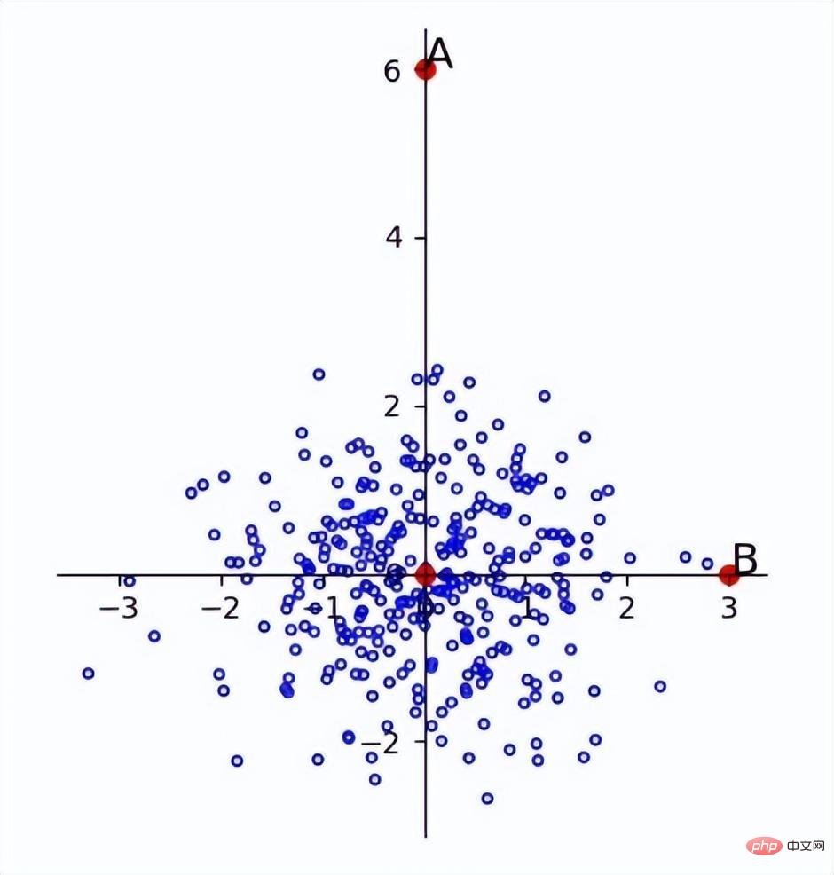
It can be seen that the outliers have been successfully separated.

The Mahalanobis distance was proposed by the Indian mathematician Mahalanobis and represents the covariance distance of the data. It is an efficient method to calculate the similarity of two unknown sample sets.

For a multivariate vector with mean

and covariance matrix Σ

, its Mahalanobis distance (the Mahalanobis distance of a single data point) is:

For The degree of difference between two random variables X and Y that obey the same distribution and whose covariance matrix is ​​Σ. The Mahalanobis distance between data points x and y is:

If the covariance matrix is ​​the identity matrix, then the Mahalanobis distance is simplified to the Euclidean distance. If the covariance matrix is ​​a diagonal matrix, then the Mahalanobis distance becomes the standardized Euclidean distance.

8. Cosine Distance

As the name suggests, cosine distance comes from the cosine of the angle in geometry, which can be used to measure the difference in the direction of two vectors. rather than distance or length. When the cosine value is 0, the two vectors are orthogonal and the included angle is 90 degrees. The smaller the angle is, the closer the cosine value is to 1 and the direction is more consistent.

In N-dimensional space, the cosine distance is:

It is worth pointing out that the cosine distance does not satisfy the triangle inequality.

9. Geodesic Distance

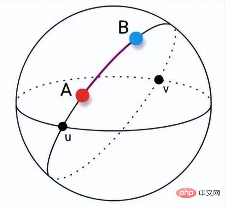
Geodesic distance originally refers to the shortest distance between the surfaces of spheres. When the feature space is a plane, the geodesic distance is the Euclidean distance. In non-Euclidean geometry, the shortest line between two points on the sphere is the great arc connecting the two points. The sides of triangles and polygons on the sphere are also composed of these great arcs.

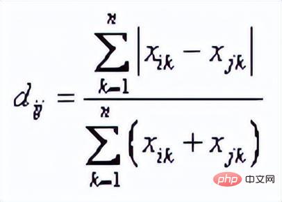
10. Bray Curtis Distance

Bray Curtis distance is mainly used Botany, Ecology and Environmental Sciences, it can be used to calculate differences between samples. The formula is:

##The value is between [0, 1]. If both vector coordinates are 0, then the value is Meaningless.

The above is the detailed content of Numerical distance based on machine learning: the distance between points in space. For more information, please follow other related articles on the PHP Chinese website!