Six clustering algorithms that data scientists must know

Currently, many applications such as Google News use clustering algorithms as the main implementation method. They can use large amounts of unlabeled data to build powerful topic clusters. This article introduces 6 types of mainstream methods from the most basic K-means clustering to powerful density-based methods. They each have their own areas of expertise and scenarios, and the basic ideas are not necessarily limited to clustering methods.

This article will start with simple and efficient K-means clustering, and then introduce mean shift clustering, density-based clustering, Gaussian mixture and maximum expectation method clustering, Hierarchical clustering and graph group detection applied to structured data. We will not only analyze the basic implementation concepts, but also give the advantages and disadvantages of each algorithm to clarify actual application scenarios.

Clustering is a machine learning technique that involves grouping data points. Given a set of data points, we can use a clustering algorithm to classify each data point into a specific group. In theory, data points belonging to the same group should have similar properties and/or characteristics, while data points belonging to different groups should have very different properties and/or characteristics. Clustering is an unsupervised learning method and a statistical data analysis technique commonly used in many fields.

K-Means (K-Means) Clustering

K-Means is probably the most well-known clustering algorithm. It is part of many introductory data science and machine learning courses. Very easy to understand and implement in code! Please see the picture below.

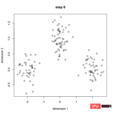
K-Means Clustering

First, we select some classes/groups and randomly initialize their respective center points. In order to work out the number of classes to use, it's a good idea to take a quick look at the data and try to identify the different groups. The center point is the location with the same length as each data point vector, which is "X" in the above image.

Classify each point by calculating the distance between the data point and the center of each group, and then classify the point in the group to which the group center is closest.

Based on these classification points, we use the mean of all vectors in the group to recalculate the group center.

Repeat these steps for a certain number of iterations, or until the group center changes little after each iteration. You could also choose to randomly initialize the group center a few times and then choose the run that seems to provide the best results.

The advantage of K-Means is that it is fast, since all we are really doing is calculating the distance between the point and the center of the group: very few calculations! So it has linear complexity O(n).

On the other hand, K-Means has some disadvantages. First, you have to choose how many groups/classes there are. This is not always done carefully, and ideally we want the clustering algorithm to help us solve the problem of how many classes to classify, since its purpose is to gain some insights from the data. K-means also starts from randomly selected cluster centers, so it may produce different clustering results in different algorithms. Therefore, results may not be reproducible and lack consistency. Other clustering methods are more consistent.

K-Medians is another clustering algorithm related to K-Means, except that instead of using the mean, the group centers are recalculated using the median vector of the group. This method is insensitive to outliers (because the median is used), but is much slower for larger data sets because a sorting is required on each iteration when calculating the median vector.

Mean Shift Clustering

Mean Shift Clustering is a sliding window-based algorithm that attempts to find dense areas of data points. This is a centroid-based algorithm, which means that its goal is to locate the center point of each group/class, which is accomplished by updating the candidate points of the center point to the mean of the points within the sliding window. These candidate windows are then filtered in a post-processing stage to eliminate near-duplications, forming the final set of center points and their corresponding groups. Please see the legend below.

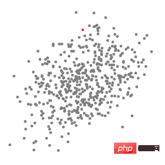
Mean shift clustering for a single sliding window

1. To explain mean shift, we will consider a set of points in a two-dimensional space, as shown in the figure above. We start with a circular sliding window centered at point C (randomly chosen) and with a core of radius r. Mean shift is a hill-climbing algorithm that involves iteratively moving toward higher density regions at each step until convergence.
2. In each iteration, the sliding window moves toward higher density areas by moving the center point toward the mean of the points within the window (hence the name). The density within a sliding window is proportional to the number of points inside it. Naturally, by moving toward the mean of the points within the window, it gradually moves toward areas of higher point density.
3. We continue to move the sliding window according to the mean until there is no direction that can accommodate more points in the kernel. Look at the picture above; we keep moving the circle until the density no longer increases (i.e. the number of points in the window).
4. The process of steps 1 to 3 is completed through many sliding windows until all points are located within one window. When multiple sliding windows overlap, the window containing the most points is retained. Then clustering is performed based on the sliding window where the data points are located.

The entire process from start to finish for all sliding windows is shown below. Each black dot represents the centroid of the sliding window, and each gray dot represents a data point.

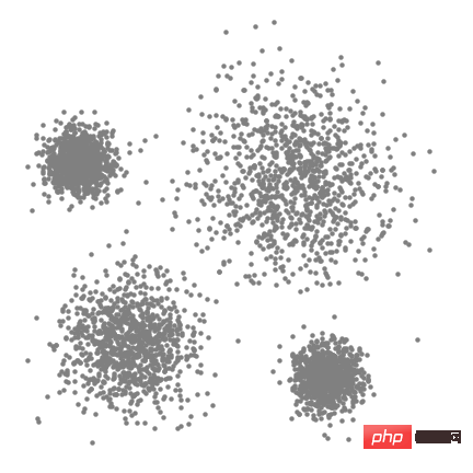
The whole process of mean shift clustering

Compared with K-means clustering, this method does not need to select the number of clusters because the mean shift automatically Discover this. This is a huge advantage. The fact that the cluster centers cluster towards the maximum point density is also very satisfying, as it is very intuitive to understand and adapt to the natural data-driven implications. The disadvantage is that the choice of window size/radius "r" may be unimportant.

Density-based clustering method (DBSCAN)

DBSCAN is a density-based clustering algorithm that is similar to mean shift but has some significant advantages. Check out another fun graphic below and let’s get started!

DBSCAN Clustering

1. DBSCAN starts from an arbitrary starting data point that has not been visited. The neighborhood of this point is extracted with distance ε (all points within ε distance are neighbor points).
2. If there are a sufficient number of points within this neighborhood (according to minPoints), the clustering process starts and the current data point becomes the first point of the new cluster. Otherwise, the point will be marked as noise (later this noise point may still become part of the cluster). In both cases, the point is marked as "Visited".
3. For the first point in a new cluster, points within its ε distance neighborhood also become part of the cluster. This process of making all points in the ε neighborhood belong to the same cluster is repeated for all new points just added to the cluster.
4. Repeat steps 2 and 3 until all points in the cluster are determined, that is, all points in the ε neighborhood of the cluster have been visited and marked.
5. Once we are done with the current cluster, a new unvisited point will be retrieved and processed, resulting in the discovery of another cluster or noise. This process is repeated until all points are marked as visited. Since all points have been visited, each point belongs to some cluster or noise.

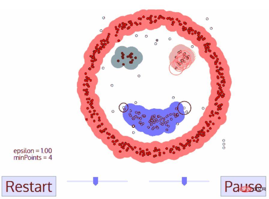
DBSCAN has many advantages over other clustering algorithms. First, it does not require a fixed number of clusters at all. It also identifies outliers as noise, unlike mean shift, which simply groups data points into clusters even if they are very different. Additionally, it is capable of finding clusters of any size and shape very well.

The main disadvantage of DBSCAN is that it does not perform as well as other clustering algorithms when the density of clusters is different. This is because the settings of the distance threshold ε and minPoints used to identify neighborhood points will change with clusters when density changes. This drawback also arises in very high-dimensional data, as the distance threshold ε again becomes difficult to estimate.

Expected Maximum (EM) Clustering with Gaussian Mixture Models (GMM)

A major drawback of K-Means is its simple use of cluster center means. From the diagram below we can see why this is not the best approach. On the left, you can see very clearly that there are two circular clusters with different radii, centered on the same mean. K-Means cannot handle this situation because the means of these clusters are very close. K-Means also fails in cases where the clusters are not circular, again due to using the mean as the cluster center.

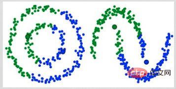
Two Failure Cases of K-Means

Gaussian Mixture Models (GMMs) give us more flexibility than K-Means. For GMMs, we assume that the data points are Gaussian distributed; this is a less restrictive assumption than using the mean to assume that they are circular. This way, we have two parameters to describe the shape of the cluster: mean and standard deviation! Taking 2D as an example, this means that the clusters can take any kind of elliptical shape (since we have standard deviations in both x and y directions). Therefore, each Gaussian distribution is assigned to a single cluster.

To find the Gaussian parameters (such as mean and standard deviation) of each cluster, we will use an optimization algorithm called Expectation Maximum (EM). Look at the diagram below, which is an example of a Gaussian fit to a cluster. We can then continue the process of maximum expectation clustering using GMMs.

EM Clustering using GMMs

1. We first choose the number of clusters (as done by K-Means) and randomly initialize each Gaussian distribution parameters of clusters. You can also try to provide a good guess for the initial parameters by taking a quick look at the data. Note however that as you can see above this is not 100% necessary as the Gaussian starts us off very poor but quickly gets optimized.
2. Given the Gaussian distribution of each cluster, calculate the probability that each data point belongs to a specific cluster. The closer a point is to the center of the Gaussian, the more likely it is to belong to that cluster. This should be intuitive since with a Gaussian distribution we assume that most of the data is closer to the center of the cluster.
3. Based on these probabilities, we calculate a new set of Gaussian distribution parameters that maximize the probability of data points within the cluster. We calculate these new parameters using a weighted sum of the data point locations, where the weight is the probability that the data point belongs to that particular cluster. To explain it visually, we can look at the image above, especially the yellow cluster, which we use as an example. The distribution starts right away on the first iteration, but we can see that most of the yellow points are on the right side of the distribution. When we calculate a probability weighted sum, even though there are some points near the center, they are mostly on the right side. Therefore, the mean of the distribution will naturally be close to these points. We can also see that most of the points are distributed "from upper right to lower left". The standard deviation is therefore changed to create an ellipse that better fits the points in order to maximize the weighted sum of the probabilities.
4. Repeat steps 2 and 3 until convergence, where the distribution changes little between iterations.

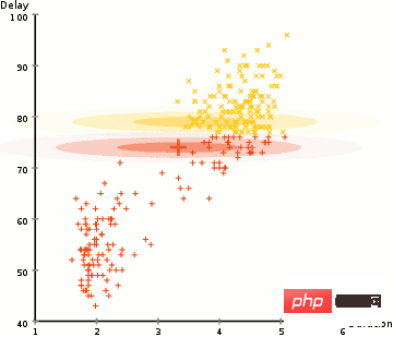
There are two key advantages to using GMMs. First, GMMs are more flexible than K-Means in terms of cluster covariance; because of the standard deviation parameter, clusters can take on any elliptical shape instead of being restricted to circles. K-Means is actually a special case of GMM, where the covariance of each cluster is close to 0 in all dimensions. Second, because GMMs use probabilities, there can be many clusters per data point. So if a data point is in the middle of two overlapping clusters, we can define its class simply by saying that X percent of it belongs to class 1 and Y percent to class 2. That is, GMMs support hybrid qualifications.

Agglomerative hierarchical clustering

Hierarchical clustering algorithms are actually divided into two categories: top-down or bottom-up. Bottom-up algorithms first treat each data point as a single cluster and then merge (or aggregate) two clusters successively until all clusters are merged into a single cluster containing all data points. Therefore, bottom-up hierarchical clustering is called agglomerative hierarchical clustering or HAC. This hierarchy of clusters is represented by a tree (or dendrogram). The root of the tree is the only cluster that collects all samples, and the leaves are the clusters with only one sample. Before going into the algorithm steps, please see the legend below.

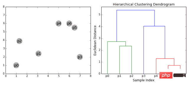
Agglomerative hierarchical clustering

1. We first treat each data point as a single cluster, i.e. if we have X data points in our data set, then we have X clusters. We then choose a distance metric that measures the distance between two clusters. As an example, we will use average linkage, which defines the distance between two clusters as the average distance between data points in the first cluster and data points in the second cluster.
2. In each iteration, we merge the two clusters into one. The two clusters to be merged should have the smallest average linkage. That is, according to the distance metric we choose, the two clusters have the smallest distance between them and are therefore the most similar and should be merged together.
3. Repeat step 2 until we reach the root of the tree, i.e. we have only one cluster containing all data points. In this way, we only need to choose when to stop merging clusters, that is, when to stop building the tree, to choose how many clusters we need in the end!

Hierarchical clustering does not require us to specify the number of clusters, we can even choose which number of clusters looks best since we are building a tree. Additionally, the algorithm is not sensitive to the choice of distance metric; they all perform equally well, whereas for other clustering algorithms the choice of distance metric is crucial. A particularly good example of hierarchical clustering methods is when the underlying data has a hierarchical structure and you want to restore the hierarchy; other clustering algorithms cannot do this. Unlike the linear complexity of K-Means and GMM, these advantages of hierarchical clustering come at the cost of lower efficiency since it has a time complexity of O(n³).

Graph Community Detection

When our data can be represented as a network or graph (graph), we can use the graph community detection method to complete clustering. In this algorithm, a graph community is usually defined as a subset of vertices that are more closely connected than other parts of the network.

Perhaps the most intuitive case is social networks. The vertices represent people, and the edges connecting the vertices represent users who are friends or fans. However, to model a system as a network, we must find a way to efficiently connect the various components. Some innovative applications of graph theory for clustering include feature extraction of image data, analysis of gene regulatory networks, etc.

Below is a simple diagram showing 8 recently viewed websites, connected based on links from their Wikipedia pages.

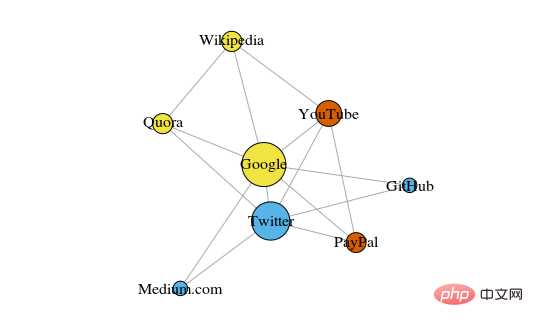
The color of these vertices indicates their group relationship, and the size is determined based on their centrality. These clusters also make sense in real life, where the yellow vertices are usually reference/search sites and the blue vertices are all online publishing sites (articles, tweets, or code).

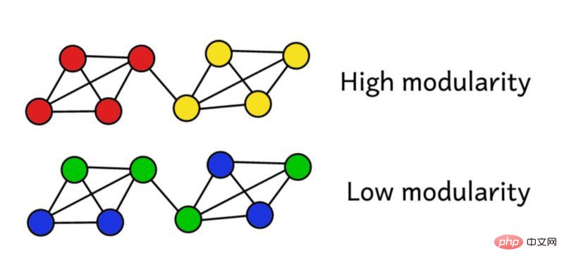
Suppose we have clustered the network into groups. We can then use this modularity score to evaluate the quality of the clustering. A higher score means we segmented the network into "accurate" groups, while a low score means our clustering is closer to random. As shown in the figure below:

Modularity can be calculated using the following formula:

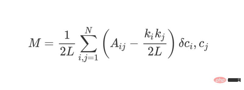
where L represents the edge in the network The quantities, k_i and k_j refer to the degree of each vertex, which can be found by adding up the terms of each row and column. Multiplying the two and dividing by 2L represents the expected number of edges between vertices i and j when the network is randomly assigned.

Overall, the terms in parentheses represent the difference between the true structure of the network and the expected structure when combined randomly. Studying its value shows that it returns the highest value when A_ij = 1 and ( k_i k_j ) / 2L is small. This means that when there is an "unexpected" edge between fixed points i and j, the resulting value is higher.

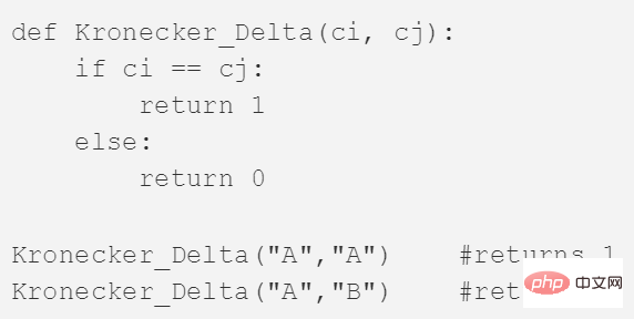
The last δc_i, c_j is the famous Kronecker δ function (Kronecker-delta function). Here is its Python explanation:

The modularity of the graph can be calculated through the above formula, and the higher the modularity, the better the degree to which the network is clustered into different groups. Therefore, the best way to cluster the network can be found by looking for maximum modularity through optimization methods.

Combinatorics tells us that for a network with only 8 vertices, there are 4140 different clustering methods. A network of 16 vertices would be clustered in over 10 billion ways. The possible clustering methods of a network with 32 vertices will exceed 128 septillion (10^21); if your network has 80 vertices, the number of possible clustering methods has exceeded the number of clustering methods in the observable universe. number of atoms.

We must therefore resort to a heuristic that works well at evaluating the clusters that yield the highest modularity scores, without trying every possibility. This is an algorithm called Fast-Greedy Modularity-Maximization, which is somewhat similar to the agglomerative hierarchical clustering algorithm described above. It’s just that Mod-Max does not fuse groups based on distance, but fuses groups based on changes in modularity.

Here's how it works:

• First initially assign each vertex to its own group, then calculate the modularity M of the entire network.
• Step 1 requires that each community pair is linked by at least one unilateral link. If two communities merge together, the algorithm calculates the resulting modularity change ΔM.
• The second step is to select the group pairs with the largest growth in ΔM and then merge them. A new modularity M is then calculated for this cluster and recorded.
• Repeat steps 1 and 2 - each time fusing the group pairs, so that the maximum gain of ΔM is finally obtained, and then record the new clustering pattern and its corresponding modularity score M.
• You can stop when all vertices are grouped into a giant cluster. The algorithm then examines the records in this process and finds the clustering pattern in which the highest M value was returned. This is the returned group structure.

Community detection is a popular research field in graph theory. Its limitations are mainly reflected in the fact that it ignores some small clusters and is only applicable to structured graph models. But this type of algorithm has very good performance in typical structured data and real network data.

Conclusion

The above are the 6 major clustering algorithms that data scientists should know! We’ll end this article by showing visualizations of various algorithms!

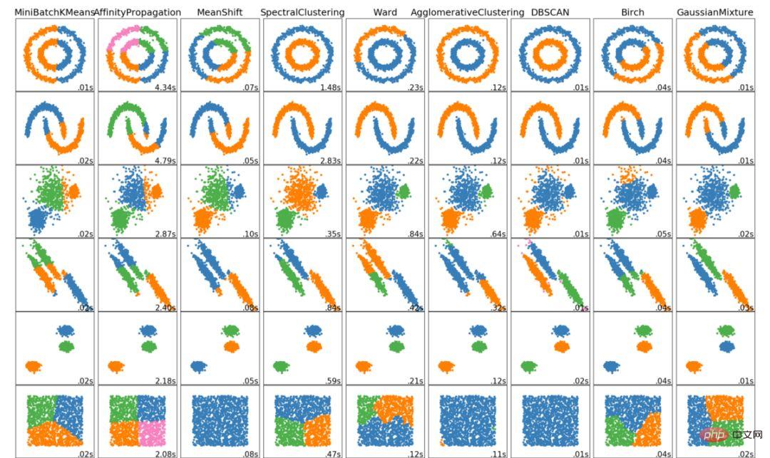
The above is the detailed content of Six clustering algorithms that data scientists must know. For more information, please follow other related articles on the PHP Chinese website!