
On the precision-recall curve, the same points are plotted with different coordinate axes. Warning: The first red dot on the left (0% recall, 100% precision) corresponds to 0 rules. The second dot on the left is the first rule, and so on.
Skope-rules uses a tree model to generate rule candidates. First build some decision trees and consider the paths from the root node to internal nodes or leaf nodes as rule candidates. These candidate rules are then filtered by some predefined criteria such as precision and recall. Only those with precision and recall above their thresholds are retained. Finally, similarity filtering is applied to select rules with sufficient diversity. In general, Skope-rules is applied to learn the underlying rules for each root cause.
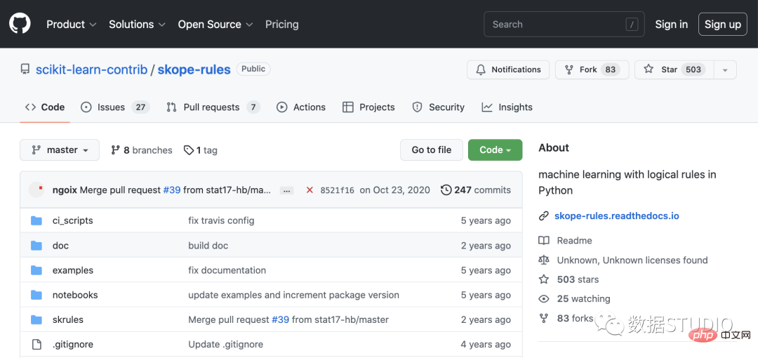
Project address: https://github.com/scikit-learn-contrib/skope-rules
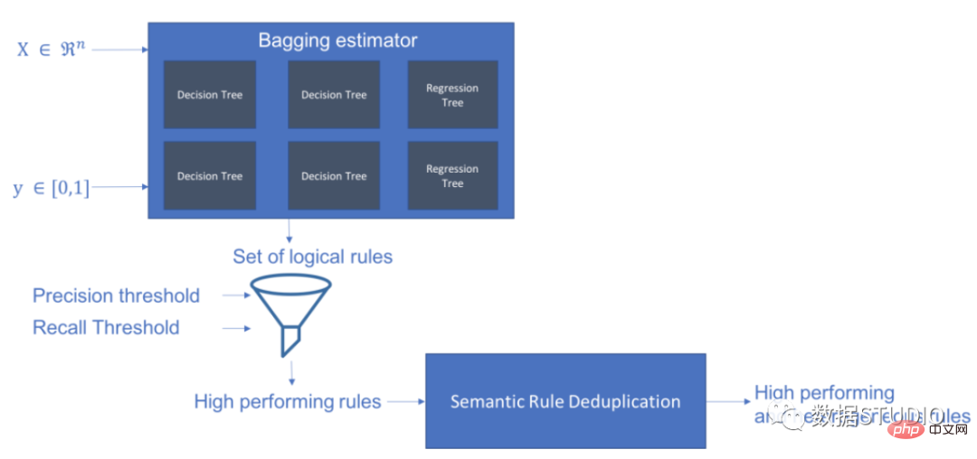
schema
You can use pip to get the latest resources:
pip install skope-rules
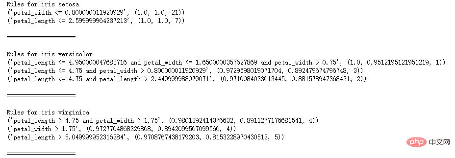
SkopeRules can be used to describe classes with logical rules:
from sklearn.datasets import load_iris
from skrules import SkopeRules
dataset = load_iris()
feature_names = ['sepal_length', 'sepal_width', 'petal_length', 'petal_width']
clf = SkopeRules(max_depth_duplicatinotallow=2,
n_estimators=30,
precision_min=0.3 ,
recall_min=0.1,
feature_names=feature_names)
for idx, species in enumerate(dataset.target_names):
X, y = dataset.data, dataset.target
clf.fit(X, y == idx)
rules = clf.rules_[0:3]
print("Rules for iris", species)
for rule in rules:
print( rule)
print()
print(20*'=')
print()
If it appears The following error:
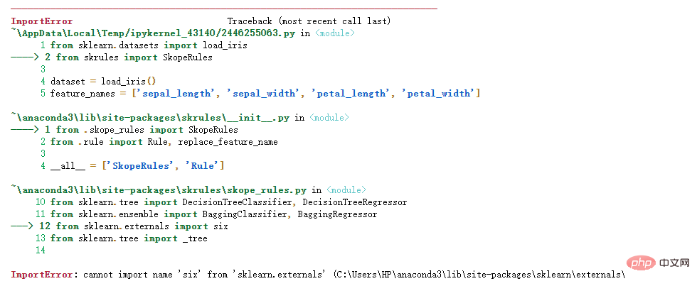
About Python import error: cannot import name 'six' from 'sklearn.externals' , Yun Duojun on Stack Overflow Found a similar question on: https://stackoverflow.com/questions/61867945/
The solution is as follows
import six
import sys
sys.modules['sklearn .externals.six'] = six
import mlrose
SkopeRules can also be used as predictors if using the "score_top_rules" method:
from sklearn.datasets import load_boston
from sklearn.metrics import precision_recall_curve
from matplotlib import pyplot as plt
from skrules import SkopeRules
dataset = load_boston()
clf = SkopeRules(max_depth_duplicatinotallow=None,
n_estimators=30,
precision_min=0.2,
recall_min=0.01 ,
feature_names=dataset.feature_names)
X, y = dataset.data, dataset.target > 25
X_train, y_train = X[:len(y)//2], y [:len(y)//2]
X_test, y_test = X[len(y)//2:], y[len(y)//2:]
clf.fit(X_train, y_train )
y_score = clf.score_top_rules(X_test) # Get a risk score for each test example
precision, recall, _ = precision_recall_curve(y_test, y_score)
plt.plot(recall, precision)
plt.xlabel('Recall')
plt.ylabel('Precision')
plt.title('Precision Recall curve')
plt.show()
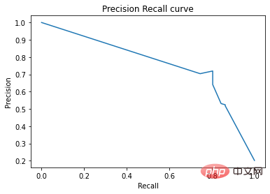
This case demonstrates the use of skope-rules on the famous Titanic data set.
skope-rules Applicability:
# Import skope-rules
from skrules import SkopeRules
# Import librairies
import pandas as pd
from sklearn.ensemble import GradientBoostingClassifier, RandomForestClassifier
from sklearn.model_selection import train_test_split
from sklearn.tree import DecisionTreeClassifier
import matplotlib.pyplot as plt
from sklearn.metrics import roc_curve, precision_recall_curve
from matplotlib import cm
import numpy as np
from sklearn.metrics import confusion_matrix
from IPython.display import display
# Import Titanic data
data = pd.read_csv('../ data/titanic-train.csv')
# Delete rows with missing ages
data = data.query('Age == Age')
# is The variable Sex creates an encoded value
data['isFemale'] = (data['Sex'] == 'female') * 1
# The variable Embarked creates an encoded value
data = pd.concat(
[data,
pd.get_dummies(data.loc[:,'Embarked'],
dummy_na=False,
prefix='Embarked',
prefix_sep='_')],
axis=1
)
# Delete unused variables
data = data.drop(['Name', 'Ticket', 'Cabin',
'PassengerId', 'Sex ', 'Embarked'],
axis = 1)
# Create training and test sets
X_train, X_test, y_train, y_test = train_test_split(
data.drop(['Survived'], axis =1),
data['Survived'],
test_size=0.25, random_state=42)
feature_names = X_train.columns
print('Column names are: ' ' '. join(feature_names.tolist()) '.')
print('Shape of training set is: ' str(X_train.shape) '.')
Column names are: Pclass Age SibSp Parch Fare
isFemale Embarked_C Embarked_Q Embarked_S.
Shape of training set is: (535, 9).
# Train a gradient boosting classifier for benchmark testing
gradient_boost_clf = GradientBoostingClassifier(random_state=42, n_estimators=30, max_depth = 5)
gradient_boost_clf.fit(X_train, y_train)
# Train a random forest classifier for benchmarking
random_forest_clf = RandomForestClassifier(random_state=42, n_estimators=30, max_depth = 5)
random_forest_clf.fit(X_train, y_train)
# Train a decision tree classifier for benchmarking
decision_tree_clf = DecisionTreeClassifier(random_state=42, max_depth = 5)
decision_tree_clf.fit(X_train, y_train)
# Train a skope-rules-boosting classifier
skope_rules_clf = SkopeRules(feature_names=feature_names, random_state= 42, n_estimators=30,
recall_min=0.05, precision_min=0.9,
max_samples=0.7,
max_depth_duplicatinotallow= 4, max_depth = 5)
skope_rules_clf.fit(X_train, y_train)
# Calculate prediction score
gradient_boost_scoring = gradient_boost_clf.predict_proba(X_test)[:, 1]
random_forest_scoring = random_forest_clf.predict_proba(X_test)[:, 1]
decision_tree_scoring = decision_tree_clf.predict_proba( X_test)[:, 1]
skope_rules_scoring = skope_rules_clf.score_top_rules(X_test)
# Get the number of created survival rules
print("Created with SkopeRules" str(len(skope_rules_clf.rules_)) "rules n")
# Print these rules
rules_explanations = [
"Under 3 years old and under 37 years old , women in first or second class. "
"Females over 3 years old traveling in first or second class and paying more than 26 euros. "
"Female who travels in first or second class and pays more than 29 euros. "
"Female who is over 39 years old and traveling in first or second class. "
]
print('The four best-performing "Titanic survival rules" are as follows:/n')
for i_rule, rule in enumerate(skope_rules_clf.rules_[:4] )
print(rule[0])
print('->' rules_explanations[i_rule] 'n')
9 rules were created using SkopeRules.
Among them The top 4 "Titanic Survival Rules" are as follows:
Age 2.5
and Pclass 0.5
-> Women under 3 years old and under 37 years old, in first or second class.
Age > 2.5 and Fare > 26.125
and Pclass 0.5
-> Women over 3 years old traveling in first or second class and paying more than 26 euros.
Fare > 29.356250762939453
and Pclass 0.5
-> Women who ride in first or second class and pay more than 29 euros.
Age > 38.5 and Pclass and isFemale > 0.5
-> Women who are over 39 years old and traveling in first or second class.
def compute_y_pred_from_query(X, rule):
score = np.zeros(X.shape[0])
X = X.reset_index(drop=True)
score[list( X.query(rule).index)] = 1
return(score)
def compute_performances_from_y_pred(y_true, y_pred, index_name='default_index'):
df = pd.DataFrame(data=
{
'precision':[sum(y_true * y_pred)/sum(y_pred)],
'recall':[sum(y_true * y_pred)/sum(y_true)]
},
index=[index_name],
columns=['precision', 'recall']
)
return(df)
def compute_train_test_query_performances(X_train, y_train, X_test, y_test , rule):
y_train_pred = compute_y_pred_from_query(X_train, rule)
y_test_pred = compute_y_pred_from_query(X_test, rule)
performances = None
performances = pd.concat([
performances,
compute_performances_from_y_pred(y_train, y_train_pred, 'train_set')],
axis=0)
performances = pd.concat([
performances,
compute_performances_from_y_pred(y_test, y_test_pred, ' test_set')],
axis=0)
return(performances)
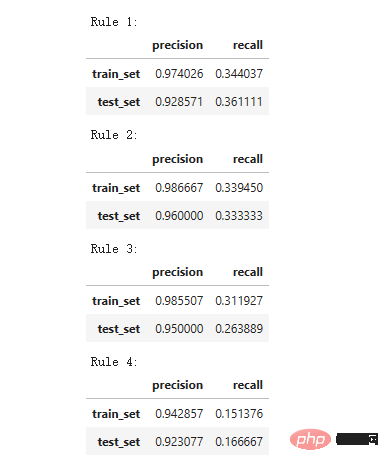
print('Precision = 0.96 means that 96% of the people determined by the rules are survivors. ')
print('Recall = 0.12 means that the survivors identified by the rule account for 12% of the total number of survivors n')
for i in range(4):
print('Rule ' str (i 1) ':')
display(compute_train_test_query_performances(X_train, y_train,
X_test, y_test,
skope_rules_clf.rules_[i][0])
)
Precision = 0.96 means that 96% of the people determined by the rules are survivors.
Recall = 0.12 means that the survivors identified by the rule account for 12% of the total survivors.
def plot_titanic_scores(y_true, scores_with_line=[], scores_with_points=[],
labels_with_line=['Gradient Boosting', 'Random Forest', 'Decision Tree'],
labels_with_points=['skope-rules']):
gradient = np.linspace(0, 1, 10)
color_list = [ cm .tab10(x) for x in gradient ]
fig, axes = plt.subplots(1, 2, figsize=(12, 5),
sharex=True, sharey=True)
ax = axes[0]
n_line = 0
for i_score, score in enumerate(scores_with_line):
n_line = n_line 1
fpr, tpr, _ = roc_curve(y_true, score)
ax.plot(fpr, tpr, linestyle='-.', c=color_list[i_score], lw=1, label=labels_with_line[i_score])
for i_score, score in enumerate(scores_with_points):
fpr , tpr, _ = roc_curve(y_true, score)
ax.scatter(fpr[:-1], tpr[:-1], c=color_list[n_line i_score], s=10, label=labels_with_points[i_score] )
ax.set_title("ROC", fnotallow=20)
ax.set_xlabel('False Positive Rate', fnotallow=18)
ax.set_ylabel('True Positive Rate (Recall)', fnotallow =18)
ax.legend(loc='lower center', fnotallow=8)
ax = axes[1]
n_line = 0
for i_score, score in enumerate(scores_with_line ):
n_line = n_line 1
precision, recall, _ = precision_recall_curve(y_true, score)
ax.step(recall, precision, linestyle='-.', c=color_list[i_score], lw =1, where='post', label=labels_with_line[i_score])
for i_score, score in enumerate(scores_with_points):
precision, recall, _ = precision_recall_curve(y_true, score)
ax.scatter (recall, precision, c=color_list[n_line i_score], s=10, label=labels_with_points[i_score])
ax.set_title("Precision-Recall", fnotallow=20)
ax.set_xlabel('Recall (True Positive Rate)', fnotallow=18)
ax.set_ylabel('Precision', fnotallow=18)
ax.legend(loc='lower center', fnotallow=8)
plt.show ()
plot_titanic_scores(y_test,
scores_with_line=[gradient_boost_scoring, random_forest_scoring, decision_tree_scoring],
scores_with_points=[skope_rules_scoring]
)
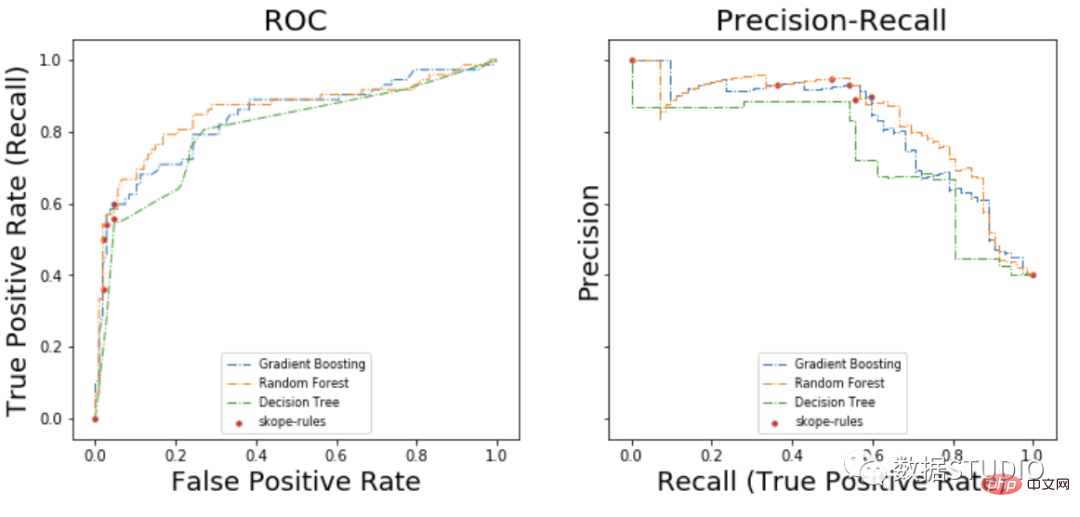
On the ROC curve, each red point corresponds to the number of activated rules (from skope-rules). For example, the lowest point is the result point of 1 rule (the best). The second lowest point is the 2 rule result point, and so on.
On the precision-recall curve, the same points are plotted with different coordinate axes. Warning: The first red dot on the left (0% recall, 100% precision) corresponds to 0 rules. The second dot on the left is the first rule, and so on.
Some conclusions can be drawn from this example.
n_rule_chosen = 4
y_pred = skope_rules_clf.predict_top_rules(X_test, n_rule_chosen)
print('The performances reached with ' str(n_rule_chosen) ' discovered rules are the following: ')
compute_performances_from_y_pred(y_test, y_pred, 'test_set')

predict_top_rules(new_data, n_r) method is used to calculate the prediction of new_data, including the first n_r items skope-rules rules.
The above is the detailed content of Increase your knowledge! Machine learning with logical rules. For more information, please follow other related articles on the PHP Chinese website!
 How to obtain the serial number of a physical hard disk under Windows
 Java performs forced type conversion
 The difference between vivox100s and x100
 How to adjust the smoke head in WIN10 system cf
 How to use fit function in Python
 What is cloud space
 How to open two WeChat accounts on Huawei mobile phone
 What are the image processing software

