How to use the MATCH() function in Excel function learning

Today we are going to talk about another family - Find the Family! Speaking of finding families, I believe the first thing that comes to mind is the VLOOKUP function. This eldest brother has been working hard in the battlefield for many years and has already become famous! I believe that friends who have been exposed to Excel have heard of it to some extent. However, what we are going to talk about today is its capable little brother - the MATCH function!

#This little brother, although his ability is not very good on his own, but when he forms a team with his big brother, the effect is quite impressive!

Let’s get to know him first

1. Who is MATCH?

MATCH is a search positioning function. What it returns is not the data itself, but the position of the data in a single column or row. It's similar to queuing up to report the number. Whichever number you stand on, MATCH the number you report! (Note: It only supports single column or single row data search~)

Function structure: MATCH (What to look for, where to find [single row or single column], search type)

Search type: 3 kind. They are represented by 0, 1, and -1 respectively. 0 indicates exact search, 1 indicates ascending search, and -1 indicates descending search.

2. Basic usage of MATCH

1. Search accurately

Give me a chestnut

We want to know where "Zhang San" ranks in the "Name" column area.

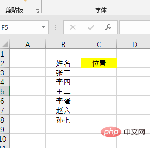
Formula:

=MATCH(B3,B$2:B$8,0)

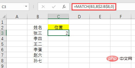
Formula analysis:

What to look for: Look for "Zhang San", so it is cell B3

Where to find it: Find it in the name column B2:B8. In order to prevent the name column area of the downward filling formula from changing, it needs to be fixed with $, that is, B$2:B$8.

Search type: 0 means precise search. Exact search does not require sorting.

2. Ascending search

Ascending search is to find the maximum value that is less than or equal to the search value and then return its location. The data must be sorted in ascending order.

Similarly give a chestnut

We want to know how many are no larger than 60.

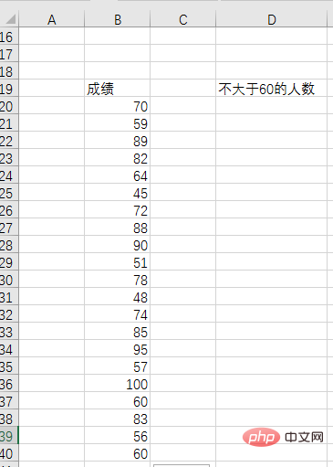
First sort the results in ascending order.

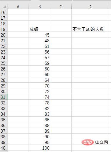
Then enter the formula in D3:=MATCH(60,B20:B40,1)

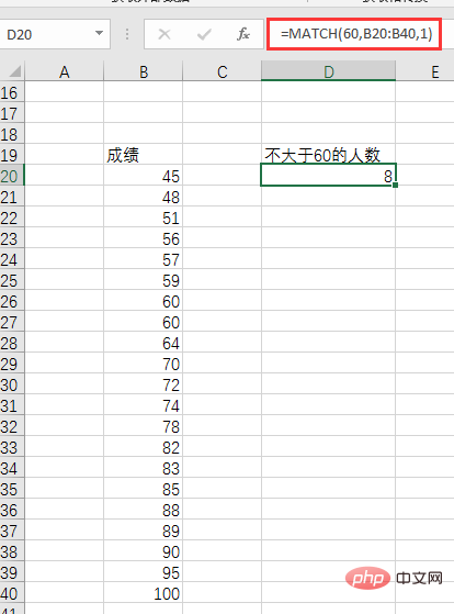
After confirmation, the number of people was 8. Obviously, after sorting in ascending order, what is returned is the position number of the last value less than or equal to 60; it can also be understood as counting the number of values not greater than 60, including all values equal to 60.

3. Descending search

Descending search is to find the minimum value that is greater than or equal to the search value and then return its location. Requirements must be sorted in descending order.

Similarly give a chestnut

We want to know how many are not less than 60. Following the above, first sort the data in descending order.

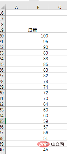
Then enter the formula in E3:=MATCH(60,B20:B40,-1)

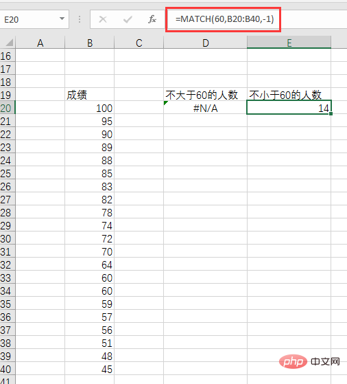
After confirmation, 14 people got no less than 60.

We got two obvious results:

(1) After descending order, an error occurs when searching in ascending order. Therefore, if you search in ascending order, you must sort in ascending order; conversely, if you search in descending order, you must sort in descending order.

(2) Descending search returns the smallest number greater than 60 or the number of positions of the first number equal to 60; it can also be understood as counting all numbers greater than 60 including the first number equal to 60 The number of values. This is different from filtering in ascending order: if there is a value that is the same as the search value, ascending order locates the last value equal to the search value, while descending order locates the first value equal to the search value.

After understanding who MATCH is and its basic usage, I guess everyone will think that MATCH is a bit useless: it is just used to return the position number, which is far from the specific value I want to find.

Because of this, the MATCH function rarely appears alone in daily work. MATCH is not discouraged. In order to win its place in the function world, it adopts an effective strategy-dancing with giants! Therefore, there are the famous VLOOKUP MATCH combination and INDEX MATCH combination.

3. Dancing with Giants

1. VLOOKUP MATCH combination

The following is a In a detailed list of scores, we need to find the total scores, average scores and grades of "Yuan Jingmi, Wang Hui, Lian Feng, and Yu Mai".

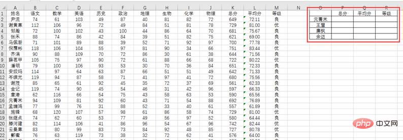
#If we use the VLOOKUP function alone, we need to frequently modify the third parameter. When checking the total score, enter the formula in cell P2:

=VLOOKUP(O2,A2:M142,11,0)

and you want to check the average score When , you need to modify the third parameter to 12, and the formula becomes:

=VLOOKUP(O2,A2:M142,12,0)

It is very convenient to use this way Trouble, how can we save trouble?

MACTH seized the opportunity to recommend itself to VLOOKUP, and replaced the third parameter with the position number of its own query "total score", "average score" and "level" in the A1:M1 row, so there is no need to modify it manually. At this time, the formula for finding the total score becomes:

=VLOOKUP($O2,$A$2:$M$142,MATCH(P$1,$A$1:$M$1,0), 0)

Then pull right to fill in and then pull down to fill in the formula to complete the query. As follows:

# Some friends may have seen our previous article "Can you use Column?" It makes the formula less dumb. ", saying that it is simpler to replace the third parameter with COLUMU:

=VLOOKUP($O2,$A$2:$M$142,COLUMN(K1),0)

You are right. The current query values are arranged continuously, and the order is consistent with the order of the score details. It is easier to use COLUMN. What if the query is based on the following two tables?

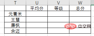
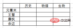
Obviously COLUMN is not suitable, but MATCH is fully qualified.

2. INDEX MATCH combination

Still check the results, as follows:

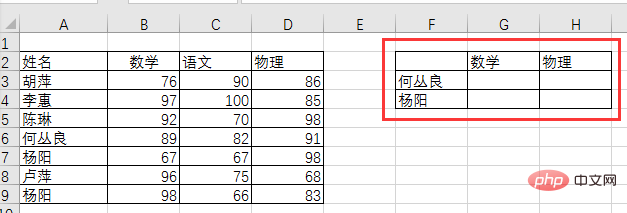
If we use INDEX alone to query scores, He Congliang’s math score query formula:=INDEX(A2:D9,5,2), physics score query formula:=INDEX(A2:D9,5,4).

INDEX query uses the specified query area as the coordinate system and queries the required values through row coordinates and column coordinates. The query area for He Congliang's grades is A2:D9, and the math score is located at the intersection of row 5 and column 2, so the formula isINDEX(A2:D9,5,2). The physics score is at the intersection of row 5 and column 4, so the formula isINDEX(A2:D9,5,4).

Querying by entering the number of rows and columns in this way is too clumsy and impractical. Therefore, MATCH took advantage of every opportunity to recommend itself to INDEX. MATCH can find the positioning value based on conditions, replacing the manual input of row and column numbers. The score query formula becomes:

=INDEX($A$2:$D$9,MATCH($F3,$A$2:$A$9,0),MATCH(G$2,$A$2 :$D$2,0))

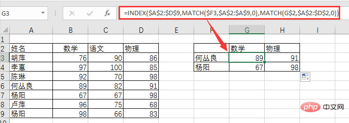
Of course you can also use the VLOOKUP MATCH combination here, the formula:

=VLOOKUP($ F3,$A$2:$D$9,MATCH(G$2,$A$2:$D$2,0),0)

What is the difference between the VLOOKUP MATCH combination and the INDEX MATCH combination? We will discuss this issue in the subsequent function class. Interested partners can think about it themselves first.

How about it? Isn’t the combination of big brother and little brother great? Therefore, the MATCH function is worthy of being the philosopher among functions! That’s it for today’s function lesson, see you next time.

Related learning recommendations:excel tutorial

The above is the detailed content of How to use the MATCH() function in Excel function learning. For more information, please follow other related articles on the PHP Chinese website!