This article brings you relevant knowledge about excel, which mainly introduces the basic syntax related knowledge of the COUNTIFS function. The syntax of this function is "COUNTIFS(criteria_range1,criteria1,[criteria_range2, criteria2]…)”, let’s take a look at it, I hope it will be helpful to everyone.

Related learning recommendations: excel tutorial
The basic syntax of the COUNTIFS function is:
COUNTIFS(criteria_range1,criteria1,[criteria_range2,criteria2]...)
Among them, criteria_range represents the condition area to be counted, criteria represents the parameters to be counted, and is used to define the Which cells are counted.
The range of each criteria_range parameter must have the same number of rows and columns. Note here that its parameters appear "in pairs". In addition, COUNTIFS supports 127 pairs of conditional statistics. You only need to understand this knowledge point. Such complex conditions will not be used in daily work.
Perform statistics on strings, numbers, and dates respectively
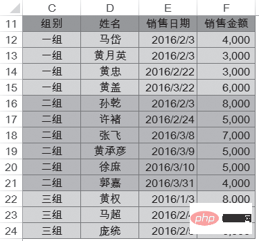
As shown in Figure 19-1, the C11:F24 cell area is the basic data source, with C as the group and D as the Name, E is listed as sales date, F is listed as sales amount, and then corresponding statistics are made on this part of the data.

First, let’s count the number of people in a group. Changing to the language of Excel, it can be translated into how many cells in column C are a "group". As shown in Figure 19-2, enter the formula in cell I12: =COUNTIFS(C12:C24,”A group”)

=COUNTIFS($C$12:$C$24,H14)

=COUNTIFS($F$12:$F$24,5000)

When doing numerical statistics, you can not only directly enter the conditions in the formula, but also place the conditions in the cells and then quote them directly. As shown in Figure 19-5, the cell areas H23:H25 are "> 5000""5000""

You can see that the statistical results are completely consistent with the previous ones. This has an advantage. If you need to modify the statistics in the future, You can modify the conditions directly in the corresponding cells of H23:H25 without modifying the formula, which is intuitive and fast. In actual work, try to consider the problem comprehensively, so that the function formula is in place in one step. In the future, you only need to modify it in the corresponding parameter area of the table.
Continue to look at a statistical data method, as shown in Figure 19-6. Enter the statistical separation point in cell H27, the number 5000, and then count "greater than", "equal to" and "less than or equal to" respectively. "Three sets of numbers. Enter the formula in cell I27:
=COUNTIFS($F$12:$F$24,”>”&H27)

Pay attention to this. Regarding the foreshadowing laid before, why are you required to write comparison operators and parameters separately? Many people will write the formula as “=COUNTIFS($F$12:$F$24,”>H27″)”. At first glance, the formula seems okay, but the result returned by this formula is 0. why? This is about talking about the issue of "activity".
H27 is not in double quotes, it maintains its "activity", which means it refers to the corresponding cell, but once it is placed in double quotes, it becomes a "mummy" , is no longer "active". ">H27" counts not the number 5000 that is greater than the number in cell H27, but the data that is greater than the three characters of "H27". In the statistics of COUNTIFS, it first determines the data type of the condition and finds that the data type is text, and the F12:F24 cell range is all numbers and no text, so the result is 0.
We use functions to reduce errors, so when you are not familiar with the function, write the comparison operator and parameters separately, and use "glue" (&) in the middle to stick them together. This can reduce 70 %mistake.
Continue to complete the other two statistics and enter the formulas in cells I28 and I29 respectively: =COUNTIFS($F$12:$F$24,”=”&H27)
=COUNTIFS( $F$12:$F$24,”
When the statistics are modified to use 3000 as the separation point, you only need to modify cell H27 to 3000, and other formulas do not need to be modified at all. can complete the work, as shown in Figure 19-7.

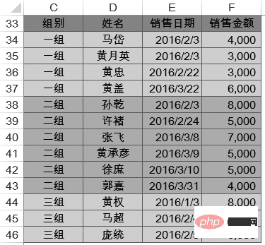
Let’s continue to look at the method of counting dates. In order to facilitate viewing the page, we establish the same data source in the C33:F46 cell area, as shown in Figure 19-8.

Count the number of people with a sales date in February 2016. Write down the formula first, and then analyze it slowly. As shown in Figure 19-9, enter the formula in cell I33: =COUNTIFS($E$34:$E$46,”>=”&”2016-2-1 ″,$E$34:$E$46,”

This function needs to pay attention to the following aspects.
(1) Review the date function discussed in Chapter 10. The essence of date and time is numbers. Counting dates in a certain interval is equivalent to counting the number between two numbers, so the method of "pinch off the beginning and remove the tail" is used.
(2) This method of quickly inputting dates must be enclosed in double quotes in English, otherwise it does not represent the date, but is just an ordinary number subtraction. If you don't master this method well, then use the DATE function in a disciplined manner, such as DATE(2016,2,1), to reduce errors.
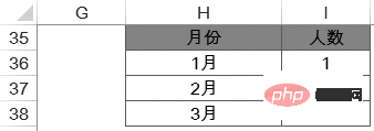
(3) The data in this data source are all dates and do not include the time part, so use “”>”&”2016-1-31″””=1st of this month (4) COUNTIFS can reference the same area multiple times. Someone asked: "The statistical formula is too long. Can you use the MONTH function to extract the month of the date, and then use the COUNTIFS function to count how many months are equal to 2?" We will know the answer after we try it. Write the formula "=COUNTIFS(MONTH(E34:E46),2)" according to this method, and then press the [Enter] key. An error message appears in the system, as shown in Figure 19-10. Figure 19-10 Formula error message There is no problem with the logic of the formula, so what exactly is the error? The result of MONTH(E34:E46) is {2;2;2;3;2;2;2;3;3;3;3;1;2;2}, which is an array, and the first parameter in COUNTIFS is criteria_range. Note that "range" means a range, so the 1st, 3rd, 5th, 7th, ... parameters of COUNTIFS do not support arrays and must be a range, that is, a range of cells must be drawn in the Excel table. Parameters that have the same requirements as it include ref and reference. With the basis of the first statistical date, we continue. When making statistics, it is impossible to manually enter every month. In most cases, January, February, March, etc. are entered in the cells, and then the corresponding statistics are completed, as shown in Figure 19-11. Enter the following formula in cell I36 and copy it down to cell I38: =COUNTIFS($E$34:$E$46,”>=”&DATE(2016,LEFTB(H36,2),1),$E $34:$E$46,” The formula looks very long, let’s interpret it step by step . The formula LEFTB(H36,2), as mentioned in Section 7.5, extracts the left 2 bytes from the month, so only the number is extracted and "1" is obtained, and this space does not affect Calculation of DATE function. DATE(2016,"1",1) returns the result "42370", which is equivalent to the date 2016-1-1. Finally, use the COUNTIFS function to complete statistics for the corresponding month. Related learning recommendations: excel tutorial
The above is the detailed content of Detailed explanation of Excel function COUNTIFS. For more information, please follow other related articles on the PHP Chinese website!
 Compare the similarities and differences between two columns of data in excel
 excel duplicate item filter color
 How to copy an Excel table to make it the same size as the original
 Excel table slash divided into two
 Excel diagonal header is divided into two
 Absolute reference input method
 java export excel
 Excel input value is illegal


