In Excel, the arrangement function is a very practical tool that can help users quickly organize data and improve work efficiency. PHP editor Youzi will share with you how to correctly use the Excel arrangement function. Through the guidance of this article, you will learn how to use arrangement functions to sort, filter and organize data, making Excel operations more convenient and efficient. Let’s master these skills together and improve work efficiency!
Rank function is most commonly used to find the ranking of a certain value in a certain area. The syntax form of the Rank function: rank (number, ref, [order]), number in the parameter after the function name is the value or cell name to be ranked (the cell must be a number), ref is the reference value area of the ranking , the order is 0 and 1, 0 means ranking from large to small (descending order), 1 means ranking from small to large (ascending order). (0 is the default, no need to enter, the result is the ranking from large to small.)
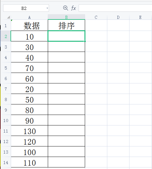
1. To give an example, I will simply take the following figure as an example and enter some data first.

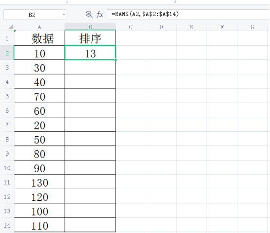
2. Enter the formula =rank($A$2,$A$2:$A$14), (you can also click the formula directly and select "Insert function", search for "rank", click OK. Then start filling in the parameters.) A2 means to determine the rank starting from the second row, and A2:A14 means the data range. You need to enter $ and use absolute references. During this process, the data area needs to be fixed to prevent the data range from changing during the pull-down process. As shown in the figure below:

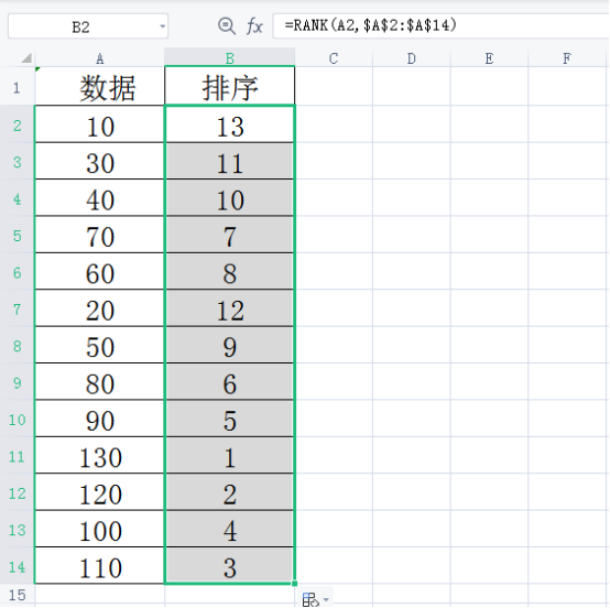
3. Then select cell B2 and place the mouse in the lower right corner. When the mouse turns into a small cross, press and hold the left button of the mouse. , pull down to cell B14, so that the ranking of all scores is displayed, as shown below:

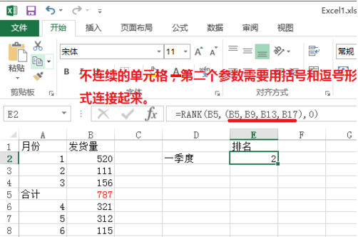
Rank function ranks discontinuous cells: discontinuous Cell, the second parameter needs to be connected with parentheses and commas. Enter the formula =rank(B5, (B5, B9, B13, B17), 0) as shown below:

When using Excel tables, many times you want Arranging a set of data to clearly and intuitively see its ranking can be done using the rank function, and it can also remove duplicate rankings.
In actual work, we will encounter various complex tables or special requirements. For example, we need to sort a set of sequences. This method is also the most common method in work, but it is relatively simple. , can handle some difficult problems. We cannot do without using Excel tables in daily work. Mastering certain software skills can help us work more efficiently.
The above is the detailed content of How to use Excel arrangement function correctly. For more information, please follow other related articles on the PHP Chinese website!
 Compare the similarities and differences between two columns of data in excel
 excel duplicate item filter color
 How to copy an Excel table to make it the same size as the original
 Excel table slash divided into two
 Excel diagonal header is divided into two
 Absolute reference input method
 java export excel
 Excel input value is illegal


