
Important unit data in Excel tables are often in the first row or column, so that people who view the table can instantly understand what the data in the table means. However, the table will inevitably be too long or too wide. After dragging the scroll wheel, the previous description data will be invisible. At this time, we can freeze the specified rows and columns of the table. Friends who don’t know how to freeze a certain row or column of a table can come here to learn more.

Tools/Materials
System version: windows10 system
Brand model: DELLInsdiron 14-3467
Method 1: Key setting
1. Select the third row
Enter the WPS excel program interface and click your mouse Left click to select the third row of the table.

2. Press the alt button
Find the alt button on your computer keyboard and press this button with your finger.

3. Press the W button
and then find the button for the letter W, press this button, and then press the F button on the keyboard twice in a row , so that your first and second rows won't move.

Method 2: Ribbon Settings
1. Select the third row of the table
Enter the excel program interface and press your Use the left mouse button to select the third row of the table.

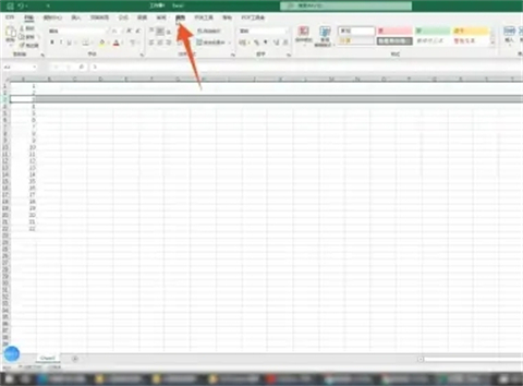
2. Click the View tab
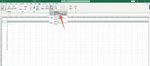
Click the View tab in the upper ribbon, and then click Freeze Pane inside.
3. Click the Freeze Pane command
Select and click the first Freeze Pane command in the pop-up menu, so that your first The first and second rows will not move.
Summary:
Method One: Button Settings
Method Two: Ribbon Settings
The above is the detailed content of How to fix specific rows and columns in a table. For more information, please follow other related articles on the PHP Chinese website!
 What are the methods of building a mobile website?
 What is the appropriate virtual memory setting?
 PathFileExists usage
 Tutorial on merging multiple words into one word
 How to clean the computer's C drive that is too full
 How to open json format
 How to create a WeChat clone on Huawei mobile phone
 out of range solution


