
AI technology is developing rapidly. Using various advanced AI models, chat robots, humanoid robots, self-driving cars, etc. can be created. AI has become the fastest growing technology, and object detection and object classification are recent trends.
This article will introduce the complete steps of building and training an image classification model from scratch using a convolutional neural network. This article will use the public Cifar-10 data set to train this model. This dataset is unique because it contains images of everyday objects like cars, airplanes, dogs, cats, etc. By training a neural network on these objects, this article will develop an intelligent system to classify these things in the real world. It contains more than 60,000 32x32 images of 10 different types of objects. By the end of this tutorial, you will have a model that can identify objects based on their visual characteristics.
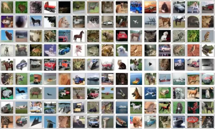
Figure 1 Dataset sample image|Picture from datasets.activeloop
This article will tell everything from the beginning, so if you haven’t learned neural networks yet The actual implementation is completely fine.
The following is the complete workflow of this tutorial:

Figure 2 Complete process
You must first install some modules to start this project. This article will use Google Colab because it provides free GPU training.
The following are the commands to install the required libraries:
<code>$ pip install tensorflow, numpy, keras, sklearn, matplotlib</code>
Import the libraries into the Python file.
<code>from numpy import *from pandas import *import matplotlib.pyplot as plotter# 将数据分成训练集和测试集。from sklearn.model_selection import train_test_split# 用来评估我们的训练模型的库。from sklearn.metrics import classification_report, confusion_matriximport keras# 加载我们的数据集。from keras.datasets import cifar10# 用于数据增量。from keras.preprocessing.image import ImageDataGenerator# 下面是一些用于训练卷积Nueral网络的层。from keras.models import Sequentialfrom keras.layers import Dense, Dropout, Activationfrom keras.layers import Conv2D, MaxPooling2D, GlobalMaxPooling2D, Flatten</code>
Now, enter the data loading step.
This section will load the data set and perform the training-test data split.
Loading and splitting data:
<code># 类的数量nc = 10(training_data, training_label), (testing_data, testing_label) = cifar10.load_data()((training_data),(validation_data),(training_label),(validation_label),) = train_test_split(training_data, training_label, test_size=0.2, random_state=42)training_data = training_data.astype("float32")testing_data = testing_data.astype("float32")validation_data = validation_data.astype("float32")</code>The cifar10 dataset is loaded directly from the Keras dataset library. And these data are also divided into training data and test data. Training data is used to train the model so that it can recognize patterns in it. While the test data is invisible to the model, it is used to check its performance, i.e. how many data points are correctly predicted relative to the total number of data points.
training_label contains the label corresponding to the image in training_data.
Then use the built-in sklearn's train_test_split function to split the training data into validation data again. Validation data were used to select and tune the final model. Finally, all training, testing and validation data are converted to 32-bit floating point numbers.
Now, the loading of the data set has been completed. In the next section, this article performs some preprocessing steps on it.
Data preprocessing is the first and most critical step in developing a machine learning model. Follow this article to find out how to do this.
<code># 归一化training_data /= 255testing_data /= 255validation_data /= 255# 热编码training_label = keras.utils.to_categorical(training_label, nc)testing_label = keras.utils.to_categorical(testing_label, nc)validation_label = keras.utils.to_categorical(validation_label, nc)# 输出数据集print("Training: ", training_data.shape, len(training_label))print("Validation: ", validation_data.shape, len(validation_label))print("Testing: ", testing_data.shape, len(testing_label))</code>Output:
<code>Training:(40000, 32, 32, 3) 40000Validation:(10000, 32, 32, 3) 10000Testing:(10000, 32, 32, 3) 10000</code>
This dataset contains images of 10 categories, each image is 32x32 pixels in size. Each pixel has a value from 0-255, and we need to normalize it between 0-1 to simplify the calculation process. After that, we will convert the categorical labels into one-hot encoded labels. This is done to convert categorical data into numerical data so that we can apply machine learning algorithms without any problem.
Now, enter the construction of CNN model.
The CNN model works in three stages. The first stage consists of convolutional layers to extract relevant features from the image. The second stage consists of pooling layers to reduce the size of the image. It also helps reduce overfitting of the model. The third stage consists of dense layers that convert the 2D image into a 1D array. Finally, this array is fed into the fully connected layer to make the final prediction.
The following is the code:
<code>model = Sequential()model.add(Conv2D(32, (3, 3), padding="same", activatinotallow="relu", input_shape=(32, 32, 3)))model.add(Conv2D(32, (3, 3), padding="same", activatinotallow="relu"))model.add(MaxPooling2D((2, 2)))model.add(Dropout(0.25))model.add(Conv2D(64, (3, 3), padding="same", activatinotallow="relu"))model.add(Conv2D(64, (3, 3), padding="same", activatinotallow="relu"))model.add(MaxPooling2D((2, 2)))model.add(Dropout(0.25))model.add(Conv2D(96, (3, 3), padding="same", activatinotallow="relu"))model.add(Conv2D(96, (3, 3), padding="same", activatinotallow="relu"))model.add(MaxPooling2D((2, 2)))model.add(Flatten())model.add(Dropout(0.4))model.add(Dense(256, activatinotallow="relu"))model.add(Dropout(0.4))model.add(Dense(128, activatinotallow="relu"))model.add(Dropout(0.4))model.add(Dense(nc, activatinotallow="softmax"))</code>
This article applies three groups of layers, each group contains two convolutional layers, a maximum pooling layer and a dropout layer. The Conv2D layer receives input_shape as (32, 32, 3), which must be the same size as the image.
Each Conv2D layer also needs an activation function, namely relu. Activation functions are used to increase nonlinearity in the system. More simply, it determines whether a neuron needs to be activated based on a certain threshold. There are many types of activation functions, such as ReLu, Tanh, Sigmoid, Softmax, etc., which use different algorithms to determine the firing of neurons.
之后,添加了平坦层和全连接层,在它们之间还有几个Dropout层。Dropout层随机地拒绝一些神经元对网层的贡献。它里面的参数定义了拒绝的程度。它主要用于避免过度拟合。
下面是一个CNN模型架构的示例图像。
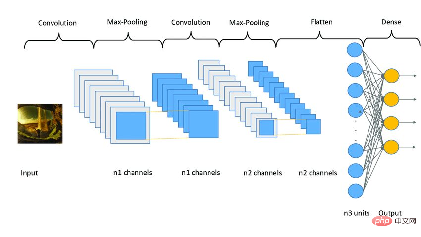
图3 Sampe CNN架构|图片来源:Researchgate
现在,本文将编译和准备训练的模型。
<code># 启动Adam优化器opt = keras.optimizers.Adam(lr=0.0001)model.compile(loss="categorical_crossentropy", optimizer=opt, metrics=["accuracy"])# 获得模型的摘要model.summary()</code>
输出:
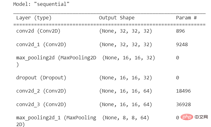
图4 模型摘要
本文使用了学习率为0.0001的Adam优化器。优化器决定了模型的行为如何响应损失函数的输出而变化。学习率是训练期间更新权重的数量或步长。它是一个可配置的超参数,不能太小或太大。
现在,本文将把模型拟合到我们的训练数据,并开始训练过程。但在此之前,本文将使用图像增强技术来增加样本图像的数量。
卷积神经网络中使用的图像增强技术将增加训练图像,而不需要新的图像。它将通过在图像中产生一定量的变化来复制图像。它可以通过将图像旋转到一定程度、添加噪声、水平或垂直翻转等方式来实现。
<code>augmentor = ImageDataGenerator(width_shift_range=0.4,height_shift_range=0.4,horizontal_flip=False,vertical_flip=True,)# 在augmentor中进行拟合augmentor.fit(training_data)# 获得历史数据history = model.fit(augmentor.flow(training_data, training_label, batch_size=32),epochs=100,validation_data=(validation_data, validation_label),)</code>
输出:
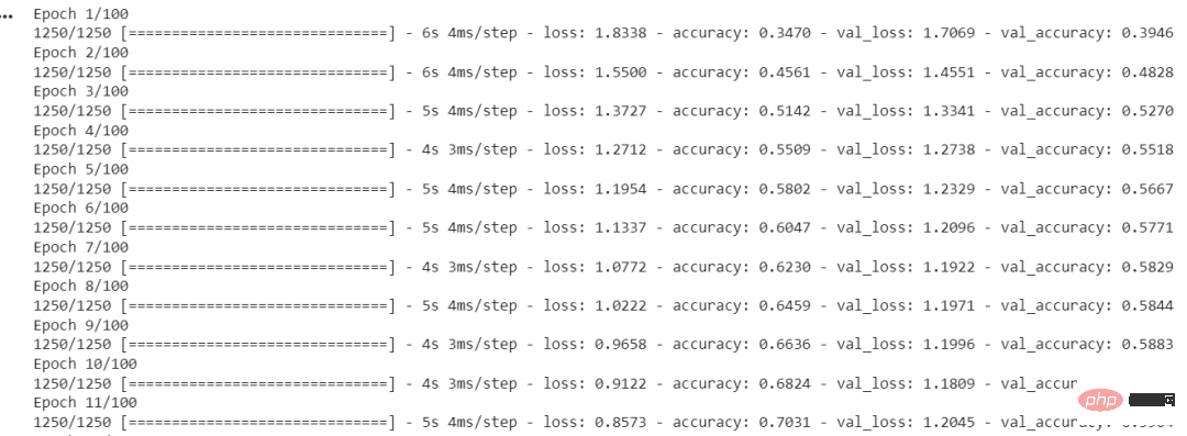
图5 每个时期的准确度和损失
ImageDataGenerator()函数用于创建增强的图像。fit()用于拟合模型。它以训练和验证数据、Batch Size和Epochs的数量作为输入。
Batch Size是在模型更新之前处理的样本数量。一个关键的超参数必须大于等于1且小于等于样本数。通常情况下,32或64被认为是最好的Batch Size。
Epochs的数量代表了所有样本在网络的前向和后向都被单独处理了多少次。100个epochs意味着整个数据集通过模型100次,模型本身运行100次。
我们的模型已经训练完毕,现在我们将评估它在测试集上的表现。
本节将在测试集上检查模型的准确性和损失。此外,本文还将绘制训练和验证数据的准确率与时间之间和损失与时间之间的关系图。
<code>model.evaluate(testing_data, testing_label)</code>
输出:
<code>313/313 [==============================] - 2s 5ms/step - loss: 0.8554 - accuracy: 0.7545[0.8554493188858032, 0.7545000195503235]</code>
本文的模型达到了75.34%的准确率,损失为0.8554。这个准确率还可以提高,因为这不是一个最先进的模型。本文用这个模型来解释建立模型的过程和流程。CNN模型的准确性取决于许多因素,如层的选择、超参数的选择、使用的数据集的类型等。
现在我们将绘制曲线来检查模型中的过度拟合情况。
<code>def acc_loss_curves(result, epochs):acc = result.history["accuracy"]# 获得损失和准确性loss = result.history["loss"]# 声明损失和准确度的值val_acc = result.history["val_accuracy"]val_loss = result.history["val_loss"]# 绘制图表plotter.figure(figsize=(15, 5))plotter.subplot(121)plotter.plot(range(1, epochs), acc[1:], label="Train_acc")plotter.plot(range(1, epochs), val_acc[1:], label="Val_acc")# 给予绘图的标题plotter.title("Accuracy over " + str(epochs) + " Epochs", size=15)plotter.legend()plotter.grid(True)# 传递值122plotter.subplot(122)# 使用训练损失plotter.plot(range(1, epochs), loss[1:], label="Train_loss")plotter.plot(range(1, epochs), val_loss[1:], label="Val_loss")# 使用 ephocsplotter.title("Loss over " + str(epochs) + " Epochs", size=15)plotter.legend()# 传递真值plotter.grid(True)# 打印图表plotter.show()acc_loss_curves(history, 100)</code>输出:
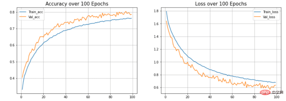
图6 准确度和损失与历时的关系
在本文的模型中,可以看到模型过度拟合测试数据集。(蓝色)线表示训练精度,(橙色)线表示验证精度。训练精度持续提高,但验证误差在20个历时后恶化。
本文展示了构建和训练卷积神经网络的整个过程。最终得到了大约75%的准确率。你可以使用超参数并使用不同的卷积层和池化层来提高准确性。你也可以尝试迁移学习,它使用预先训练好的模型,如ResNet或VGGNet,并在某些情况下可以提供非常好的准确性。
The above is the detailed content of It's easy to build and train your first neural network with TensorFlow and Keras. For more information, please follow other related articles on the PHP Chinese website!


