11 common classification feature encoding techniques
The machine learning algorithm only accepts numerical input, so if we encounter categorical features, we will encode the categorical features. This article summarizes 11 common categorical variable encoding methods.

1. ONE HOT ENCODING
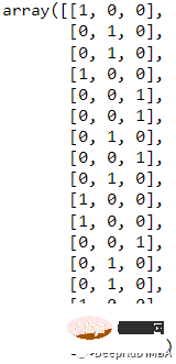
The most popular and commonly used encoding method is One Hot Enoding. A single variable with n observations and d distinct values is converted into d binary variables with n observations, each binary variable is identified by a bit (0, 1).
For example:

After encoding
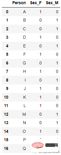
new_df=pd.get_dummies(columns=[‘Sex’], data=df)

from sklearn.preprocessing import LabelEncoder
 le=LabelEncoder()
 df[‘Sex’]=le.fit_transform(df[‘Sex’])

##
from sklearn.preprocessing import LabelBinarizer
 lb = LabelBinarizer()
 new_df[‘Sex’]=lb.fit_transform(df[‘Sex’])
 4. Leave one out Encoding
 When Leave One Out is encoded, all records with the same value for the target categorical feature variable are averaged to determine the mean of the target variable. The encoding algorithm differs slightly between the training and test datasets. Because the feature records considered for classification are excluded from the training data set, it is called "Leave One Out".
Specific values of specific categorical variables are coded as follows.
ci = (Σj != i tj / (n — 1 + R)) x (1 + εi) where
 ci = encoded value for ith record
 tj = target variable value for jth record
 n = number of records with the same categorical variable value
 R = regularization factor
 εi = zero mean random variable with normal distribution N(0, s)
For example, the following data:
 After encoding:
 To demonstrate this encoding process , we create the data set:
import pandas as pd;
 data = [[‘1’, 120], [‘2’, 120], [‘3’, 140],
 [‘2’, 100], [‘3’, 70], [‘1’, 100],[‘2’, 60],
 [‘3’, 110], [‘1’, 100],[‘3’, 70] ]
 df = pd.DataFrame(data, columns = [‘Dept’,’Yearly Salary’])
and then encode:
import category_encoders as ce
 tenc=ce.TargetEncoder()
 df_dep=tenc.fit_transform(df[‘Dept’],df[‘Yearly Salary’])
 df_dep=df_dep.rename({‘Dept’:’Value’}, axis=1)
df_new = df.join(df_dep)This way we get the above result.
5. Hashing
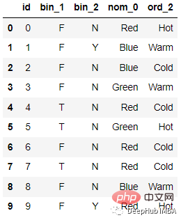
When using the hash function, the string will be converted into a unique hash value. Because it uses very little memory and can handle more categorical data. Feature hashing is an effective method for managing sparse high-dimensional features in machine learning. It is suitable for online learning scenarios and has the characteristics of fast, simple, efficient and fast.
For example, the following data:
 After encoding
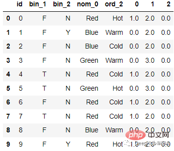 The code is as follows:
from sklearn.feature_extraction import FeatureHasher
 # n_features contains the number of bits you want in your hash value.
 h = FeatureHasher(n_features = 3, input_type =’string’)
 # transforming the column after fitting
 hashed_Feature = h.fit_transform(df[‘nom_0’])
 hashed_Feature = hashed_Feature.toarray()
 df = pd.concat([df, pd.DataFrame(hashed_Feature)], axis = 1)
 df.head(10)
6. Weight of Evidence Encoding
(WoE) The main goal of development is to create a predictive model for assessing loan default risk in the credit and financial industry. The extent to which evidence supports or refutes a theory depends on its weight of evidence, or WOE.
 If P(Goods) / P(Bads) = 1, then WoE is 0. If the outcome for this group is random, then P(Bads) > P(Goods), the odds ratio is 1, and the weight of evidence (WoE) is 0. If P(Goods) > P(bad) in a group, then WoE is greater than 0.
因为Logit转换只是概率的对数,或ln(P(Goods)/P(bad)),所以WoE非常适合于逻辑回归。当在逻辑回归中使用wo编码的预测因子时,预测因子被处理成与编码到相同的尺度,这样可以直接比较线性逻辑回归方程中的变量。
例如下面的数据
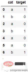
会被编码为:

代码如下:
from category_encoders import WOEEncoder
 df = pd.DataFrame({‘cat’: [‘a’, ‘b’, ‘a’, ‘b’, ‘a’, ‘a’, ‘b’, ‘c’, ‘c’], ‘target’: [1, 0, 0, 1, 0, 0, 1, 1, 0]})
 woe = WOEEncoder(cols=[‘cat’], random_state=42)
 X = df[‘cat’]
 y = df.target
encoded_df = woe.fit_transform(X, y)7、Helmert Encoding
Helmert Encoding将一个级别的因变量的平均值与该编码中所有先前水平的因变量的平均值进行比较。
反向 Helmert 编码是类别编码器中变体的另一个名称。它将因变量的特定水平平均值与其所有先前水平的水平的平均值进行比较。

会被编码为

代码如下:
import category_encoders as ce
 encoder=ce.HelmertEncoder(cols=’Dept’)
 new_df=encoder.fit_transform(df[‘Dept’])
 new_hdf=pd.concat([df,new_df], axis=1)
 new_hdf
8、Cat Boost Encoding
是CatBoost编码器试图解决的是目标泄漏问题,除了目标编码外,还使用了一个排序概念。它的工作原理与时间序列数据验证类似。当前特征的目标概率仅从它之前的行(观测值)计算,这意味着目标统计值依赖于观测历史。

TargetCount:某个类别特性的目标值的总和(到当前为止)。
Prior:它的值是恒定的,用(数据集中的观察总数(即行))/(整个数据集中的目标值之和)表示。
featucalculate:到目前为止已经看到的、具有与此相同值的分类特征的总数。
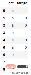
编码后的结果如下:
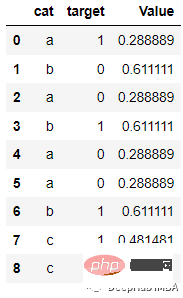
代码:
import category_encoders
 category_encoders.cat_boost.CatBoostEncoder(verbose=0,
 cols=None, drop_invariant=False, return_df=True,
 handle_unknown=’value’, handle_missing=’value’,
 random_state=None, sigma=None, a=1)

 target = df[[‘target’]]
 train = df.drop(‘target’, axis = 1)

 # Define catboost encoder
 cbe_encoder = ce.cat_boost.CatBoostEncoder()

 # Fit encoder and transform the features
 cbe_encoder.fit(train, target)
 train_cbe = cbe_encoder.transform(train)
9、James Stein Encoding
James-Stein 为特征值提供以下加权平均值:
- 观察到的特征值的平均目标值。
- 平均期望值(与特征值无关)。
James-Stein 编码器将平均值缩小到全局的平均值。该编码器是基于目标的。但是James-Stein 估计器有缺点:它只支持正态分布。
它只能在给定正态分布的情况下定义(实时情况并非如此)。为了防止这种情况,我们可以使用 beta 分布或使用对数-比值比转换二元目标,就像在 WOE 编码器中所做的那样(默认使用它,因为它很简单)。
10、M Estimator Encoding:
Target Encoder的一个更直接的变体是M Estimator Encoding。它只包含一个超参数m,它代表正则化幂。m值越大收缩越强。建议m的取值范围为1 ~ 100。
11、 Sum Encoder
Sum Encoder将类别列的特定级别的因变量(目标)的平均值与目标的总体平均值进行比较。在线性回归(LR)的模型中,Sum Encoder和ONE HOT ENCODING都是常用的方法。两种模型对LR系数的解释是不同的,Sum Encoder模型的截距代表了总体平均值(在所有条件下),而系数很容易被理解为主要效应。在OHE模型中,截距代表基线条件的平均值,系数代表简单效应(一个特定条件与基线之间的差)。
最后,在编码中我们用到了一个非常好用的Python包 “category-encoders”它还提供了其他的编码方法,如果你对他感兴趣,请查看它的官方文档:
http://contrib.scikit-learn.org/category_encoders/
The above is the detailed content of 11 common classification feature encoding techniques. For more information, please follow other related articles on the PHP Chinese website!

Hot AI Tools

Undresser.AI Undress
AI-powered app for creating realistic nude photos

AI Clothes Remover
Online AI tool for removing clothes from photos.

Undress AI Tool
Undress images for free

Clothoff.io
AI clothes remover

AI Hentai Generator
Generate AI Hentai for free.

Hot Article

Hot Tools

Notepad++7.3.1
Easy-to-use and free code editor

SublimeText3 Chinese version
Chinese version, very easy to use

Zend Studio 13.0.1
Powerful PHP integrated development environment

Dreamweaver CS6
Visual web development tools

SublimeText3 Mac version
God-level code editing software (SublimeText3)

Hot Topics
 1377
1377
 52
52
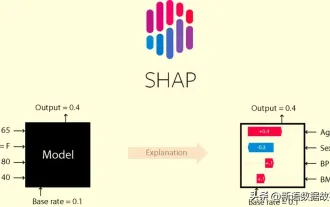 This article will take you to understand SHAP: model explanation for machine learning
Jun 01, 2024 am 10:58 AM
In the fields of machine learning and data science, model interpretability has always been a focus of researchers and practitioners. With the widespread application of complex models such as deep learning and ensemble methods, understanding the model's decision-making process has become particularly important. Explainable AI|XAI helps build trust and confidence in machine learning models by increasing the transparency of the model. Improving model transparency can be achieved through methods such as the widespread use of multiple complex models, as well as the decision-making processes used to explain the models. These methods include feature importance analysis, model prediction interval estimation, local interpretability algorithms, etc. Feature importance analysis can explain the decision-making process of a model by evaluating the degree of influence of the model on the input features. Model prediction interval estimate
 Implementing Machine Learning Algorithms in C++: Common Challenges and Solutions
Jun 03, 2024 pm 01:25 PM
Common challenges faced by machine learning algorithms in C++ include memory management, multi-threading, performance optimization, and maintainability. Solutions include using smart pointers, modern threading libraries, SIMD instructions and third-party libraries, as well as following coding style guidelines and using automation tools. Practical cases show how to use the Eigen library to implement linear regression algorithms, effectively manage memory and use high-performance matrix operations.
 Explainable AI: Explaining complex AI/ML models
Jun 03, 2024 pm 10:08 PM
Translator | Reviewed by Li Rui | Chonglou Artificial intelligence (AI) and machine learning (ML) models are becoming increasingly complex today, and the output produced by these models is a black box – unable to be explained to stakeholders. Explainable AI (XAI) aims to solve this problem by enabling stakeholders to understand how these models work, ensuring they understand how these models actually make decisions, and ensuring transparency in AI systems, Trust and accountability to address this issue. This article explores various explainable artificial intelligence (XAI) techniques to illustrate their underlying principles. Several reasons why explainable AI is crucial Trust and transparency: For AI systems to be widely accepted and trusted, users need to understand how decisions are made
 Improved detection algorithm: for target detection in high-resolution optical remote sensing images
Jun 06, 2024 pm 12:33 PM
01 Outlook Summary Currently, it is difficult to achieve an appropriate balance between detection efficiency and detection results. We have developed an enhanced YOLOv5 algorithm for target detection in high-resolution optical remote sensing images, using multi-layer feature pyramids, multi-detection head strategies and hybrid attention modules to improve the effect of the target detection network in optical remote sensing images. According to the SIMD data set, the mAP of the new algorithm is 2.2% better than YOLOv5 and 8.48% better than YOLOX, achieving a better balance between detection results and speed. 02 Background & Motivation With the rapid development of remote sensing technology, high-resolution optical remote sensing images have been used to describe many objects on the earth’s surface, including aircraft, cars, buildings, etc. Object detection in the interpretation of remote sensing images
 Is Flash Attention stable? Meta and Harvard found that their model weight deviations fluctuated by orders of magnitude
May 30, 2024 pm 01:24 PM
MetaFAIR teamed up with Harvard to provide a new research framework for optimizing the data bias generated when large-scale machine learning is performed. It is known that the training of large language models often takes months and uses hundreds or even thousands of GPUs. Taking the LLaMA270B model as an example, its training requires a total of 1,720,320 GPU hours. Training large models presents unique systemic challenges due to the scale and complexity of these workloads. Recently, many institutions have reported instability in the training process when training SOTA generative AI models. They usually appear in the form of loss spikes. For example, Google's PaLM model experienced up to 20 loss spikes during the training process. Numerical bias is the root cause of this training inaccuracy,
 Five schools of machine learning you don't know about
Jun 05, 2024 pm 08:51 PM
Machine learning is an important branch of artificial intelligence that gives computers the ability to learn from data and improve their capabilities without being explicitly programmed. Machine learning has a wide range of applications in various fields, from image recognition and natural language processing to recommendation systems and fraud detection, and it is changing the way we live. There are many different methods and theories in the field of machine learning, among which the five most influential methods are called the "Five Schools of Machine Learning". The five major schools are the symbolic school, the connectionist school, the evolutionary school, the Bayesian school and the analogy school. 1. Symbolism, also known as symbolism, emphasizes the use of symbols for logical reasoning and expression of knowledge. This school of thought believes that learning is a process of reverse deduction, through existing
 Machine Learning in C++: A Guide to Implementing Common Machine Learning Algorithms in C++
Jun 03, 2024 pm 07:33 PM
In C++, the implementation of machine learning algorithms includes: Linear regression: used to predict continuous variables. The steps include loading data, calculating weights and biases, updating parameters and prediction. Logistic regression: used to predict discrete variables. The process is similar to linear regression, but uses the sigmoid function for prediction. Support Vector Machine: A powerful classification and regression algorithm that involves computing support vectors and predicting labels.
 Outlook on future trends of Golang technology in machine learning
May 08, 2024 am 10:15 AM
The application potential of Go language in the field of machine learning is huge. Its advantages are: Concurrency: It supports parallel programming and is suitable for computationally intensive operations in machine learning tasks. Efficiency: The garbage collector and language features ensure that the code is efficient, even when processing large data sets. Ease of use: The syntax is concise, making it easy to learn and write machine learning applications.


