
Julia is a highly abstract dynamic programming language. Although it is a general-purpose language capable of developing all programs, it has several features that make it well suited for scientific computing and numerical calculations. Python emerged as a simple object-oriented programming language in the early 1990s and has evolved significantly today. This article will discuss their performance in neural networks and machine learning.
Julia's architecture is mainly characterized by parametric polymorphism in dynamic languages and the programming paradigm of multiple dispatch. It allows concurrent, parallel and distributed computing with or without the message passing interface (MPI) or built-in "OpenMP-style" threads, as well as direct calls to C and FORTRAN libraries without additional code. Julia uses a just-in-time (JIT) compiler, which the Julia community calls "just-ahead-of-time (JAOT)" because it compiles all code to machine code by default before running.
Unlike Python, Julia is designed for statistics and machine learning. Julia can perform linear algebra operations quickly, but Python is very slow. This is because Python was never designed to accommodate the matrices and equations used in machine learning. Python itself isn't bad, especially Numpy, but without using packages, Julia feels more tailor-made for math. Julia's operators are more R-like than Python's, which is a significant advantage. Most linear algebra operations can be performed with less time and effort.
As we all know, Python has dominated the fields of machine learning and data science in recent years. Because in Python we can use a variety of third-party libraries to help us write machine learning code. Although Python has so many advantages, it still has one major disadvantage - it is an interpreted language and is very slow. Now is the age of data. The more data we have, the longer it takes us to process it, which is why Julia appears.
So far, research work on Julia has focused on topics such as high performance or Julia's scientific computing capabilities. But here, we will discuss about Julia’s ability to efficiently handle not only complex scientific calculations but also business-based problems, as well as machine learning and neural networks like Python.
Julia is as simple as Python, but it is a compiled language like C. First let's test how much faster Julia is than Python. To do this, we first test them on some simple programs and then come to the focus of our experiments, testing their machine learning and deep learning capabilities.
Both Julia and Python provide many libraries and open source benchmarking tools. For benchmarking and calculating times in Julia we used the CPUTime and time libraries; for Python we also used the time module.
At first we tried simple arithmetic operations, but since these operations did not make much of a time difference, we decided to compare the time difference of matrix multiplication. We create two (10 * 10) matrices of random floating point numbers and perform a dot product on them. As we all know, Python has a Numpy library, which is often used to calculate matrices and vectors. Julia also has a LinearAlgebra library, which is often used to calculate matrices and vectors. Therefore, we compared the time consuming of matrix multiplication with and without the library respectively. All source code used in this article has been placed in the GitHub repository. Given below is a 10×10 matrix multiplication program written in Julia:
@time LinearAlgebra.mul!(c,x,y)


function MM()

x = rand(Float64,(10,10))

y = rand(Float64,(10,10))

c = zeros(10,10)


for i in range(1,10)

for j in range(1,10)

for k in range(1,10)

c[i,j] += x[i,k]*y[k,j]

end

end

end

end

@time MM


0.000001 seconds

MM (generic function with 1 method)
Julia took 0.000017 seconds using the library and 0.000001 seconds using a loop.
Use Python to write the same matrix multiplication program as follows. From the results, it can be found that the program using the library takes less time than not using the library:
import numpy as np

import time as t

x = np.random.rand(10,10)

y = np.random.rand(10,10)

start = t.time()

z = np.dot(x, y)

print(“Time = “,t.time()-start)

Time = 0.001316070556640625


import random

import time as t

l = 0

h= 10

cols = 10

rows= 10


choices = list (map(float, range(l,h)))

x = [random.choices (choices , k=cols) for _ in range(rows)]

y = [random.choices (choices , k=cols) for _ in range(rows)]


result = [([0]*cols) for i in range (rows)]


start = t.time()


for i in range(len(x)):

for j in range(len(y[0])):

for k in range(len(result)):

result[i][j] += x[i][k] * y[k][j]


print(result)

print(“Time = “, t.time()-start)


Time = 0.0015912055969238281
Python takes 0.0013 seconds using the library and 0.0015 seconds using the loop.
The next experiment we performed was a linear search on a hundred thousand randomly generated numbers. Two methods are used here, one is to use for loop, and the other is to use operators. We performed 1000 searches using integers from 1 to 1000, and as you can see in the output below, we also printed how many integers we found in the dataset. Given below are the times when using a loop and using the IN operator. Here we use the median of 3 CPU run times.
The program written in Julia and the running results are as follows:
(LCTT translation annotation: Julia code is missing in the original text here)
The program written in Python and the running results are as follows:
import numpy as np

import time as t

x = np.random.rand(10,10)

y = np.random.rand(10,10)

start = t.time()

z = np.dot(x, y)

print(“Time = “,t.time()-start)

Time = 0.001316070556640625


import random

import time as t

l = 0

h= 10

cols = 10

rows= 10


choices = list (map(float, range(l,h)))

x = [random.choices (choices , k=cols) for _ in range(rows)]

y = [random.choices (choices , k=cols) for _ in range(rows)]


result = [([0]*cols) for i in range (rows)]


start = t.time()


for i in range(len(x)):

for j in range(len(y[0])):

for k in range(len(result)):

result[i][j] += x[i][k] * y[k][j]


print(result)

print(“Time = “, t.time()-start)


Time = 0.0015912055969238281
FOR_SEARCH:

Elapsed CPU time: 16.420260511 seconds

matches: 550

Elapsed CPU time: 16.140975079 seconds

matches: 550

Elapsed CPU time: 16.49639576 seconds

matches: 550


IN:

Elapsed CPU time: 6.446583343 seconds

matches: 550

Elapsed CPU time: 6.216615487 seconds

matches: 550

Elapsed CPU time: 6.296716556 seconds

matches: 550
From the above results, using loops and operators in Julia does not produce a significant time difference. But looping in Python takes almost three times longer than operator IN. Interestingly, in both cases, Julia is significantly faster than Python.
The next experiment is to test the machine learning algorithm. We chose linear regression, one of the most common and simplest machine learning algorithms, using a simple data set. We used a data set "Head Brain" containing 237 pieces of data. The two columns of the data set are "HeadSize" and "BrainWeight". Next, we use the “head size” data to calculate the “brain weight”. In both Python and Julia, we did not use third-party libraries, but implemented the linear regression algorithm from scratch.
Julia:
GC.gc()

@CPUtime begin

linear_reg()

end

elapsed CPU time: 0.000718 seconds
Python:
gc.collect()

start = process_time()

linear_reg()

end = process_time()


print(end-start)

elapsed time: 0.007180344000000005
Times taken for Julia and Python are given above.
Next, we conducted experiments on the most common machine learning algorithm, namely logistic regression, using libraries in both languages. For Python we use the most common library sklearn; for Julia we use the GLM library. The dataset we use here is about bank customers and contains 10,000 data entries. The target variable is a binary variable that distinguishes whether a consumer continues to use a bank account.
The time it takes for Julia to perform logistic regression is given below:
@time log_rec()

0.027746 seconds (3.32 k allocations: 10.947 MiB)
The time it takes for Python to perform logistic regression is given below:
gc.collect()

start = process_time()

LogReg()

end = process_time()

print(end-start)


Accuracy : 0.8068

0.34901400000000005
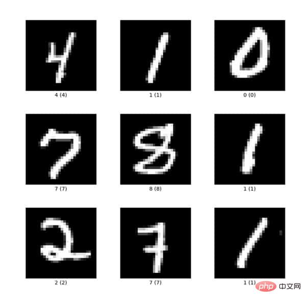
在各种程序和数据集上测试这两种语言后,我们在神经网络上使用 MNIST 数据集继续测试它们。该数据集包含从零到九的手绘数字的灰度图像。每张图像为 28×28 像素。每个像素值表示该像素的亮度或暗度,该值是包含 0 到 255 之间的整数。该数据还包含一个标签列,该列表示在相关图像中绘制的数字。

Figure 1: Example of MNIST data set
图 1 是 MNIST 数据集的示例。
对两种语言我们都建立了一个简单的神经网络来测试它们耗费的时间。神经网络的结构如下:
Input ---> Hidden layer ---> Output
该神经网络包含了一个输入层、隐层还有输出层。为了避免神经网络的复杂度过高,我们对数据集没有进行任何的预处理工作。在 Julia 和 Python 中我们都进行了40次训练并比较它们的时间差异。

Figure 2: Julia takes 5.76 seconds in a neural network
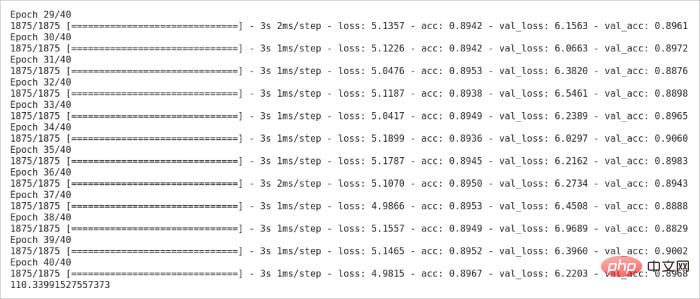
在 Julia 中,Flux 库通常被用于建立神经网络;在 Python 中我们常使用 Keras 库。图 2 展示了 Julia 在神经网络上的耗时。图 3 展示了 Python 的神经网络经过了若干次训练的耗时。

Figure 3: Python takes 110.3 seconds in a neural network
这个结果展示了 Julia 和 Python 在处理神经网络时存在巨大的时间差异。
表 1 总结了此次实验的测试结果并计算了 Julia 和 Python 时间差异的百分比。
实验 |
Julia(秒) |
Python(秒) |
时间差(%) |
矩阵乘法(不使用库) |
0.000001 |
0.0015 |
99.9 |
| ##Matrix multiplication ( Using library) |
0.000017 |
0.0013 |
98.69 |
| Linear search (using loops) |
0.42
|
16.4 |
97.43 |
|
|
|
||
|
|
|
|
| 0.025 |
0.34901 |
##92.83 |
| Neural Network |
5.76 | ##110.3 | 94.77
The above is the detailed content of Julia or Python, which one is faster?. For more information, please follow other related articles on the PHP Chinese website!


