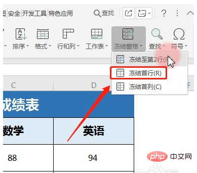
How to set fixed rows

How to set fixed rows: First open the document; then find "Start" in the menu bar and click "Freeze Panes"; finally select [Freeze First Row] or click [Freeze Panes- Freeze to the second row].

The operating environment of this article: Windows 7 system, DELL G3 computer, Microsoft Office Excel 2010 version.

First open the document, find "Start" in the menu bar, and click "Freeze Panes"

There are three modes here, the ones we generally use are [Freeze first row], we only need to select the first row, and then click [Freeze first row] to make the first row display at the top

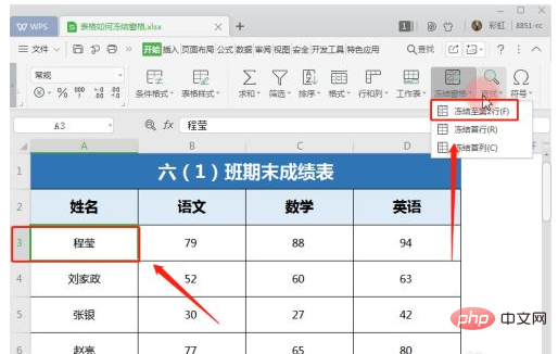
For example, I need to freeze now" "A1, A2" two rows, then I must select the "A3" cell,

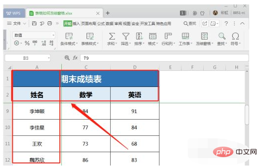
Click "Freeze Panes" - "Freeze to the second row", and then drag Scroll bar, the first two rows will not be covered;

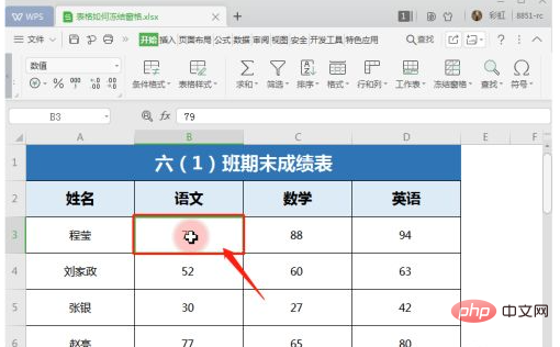
#If you want to freeze a row and a column at the same time, for example, you want to freeze row A2 and column A1 at the same time.

First you need to find the cells that are connected with them, click on cell B3,

Click "Freeze Pane" - "Freeze to No. 2 rows and column A" is enough.

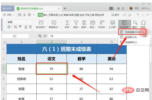
In this way, the columns and rows we want to set are fixed! [Recommended learning:Excel tutorial]

The above is the detailed content of How to set fixed rows. For more information, please follow other related articles on the PHP Chinese website!