
Recommended tutorial: Excel tutorial
Take the 2007 version of EXCEL as an example, as shown in the figure below Use the VLOOKUP function to perform batch searches and return the amount corresponding to the search target.
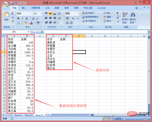
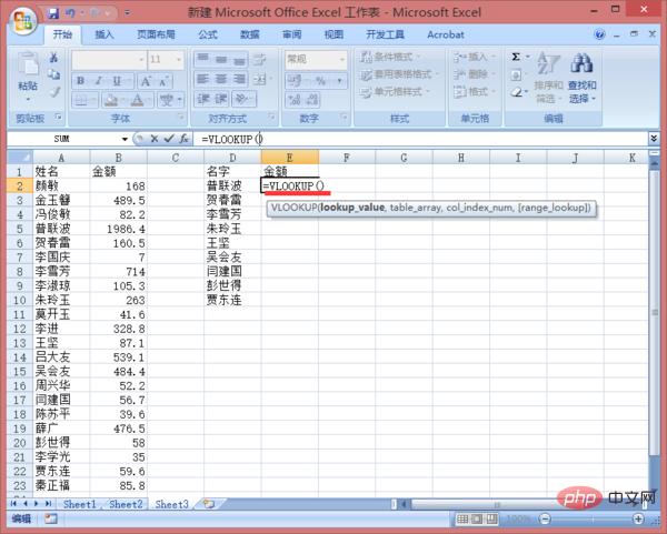
1. Open the Excel worksheet and enter the search function VLOOKUP in cell E2, that is: =VLOOKUP().
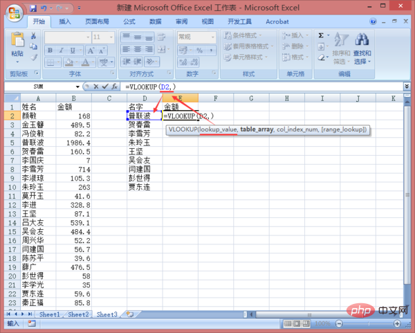
2. Enter the first parameter of the VLOOKUP function: lookup_value, the value to be looked up, also known as the lookup value, that is, the unit where the search target is located. Grid D2, as shown in the figure below.
3. Enter the second parameter of the VLOOKUP function: table_array to check the area where the value is located, which is the area range where the data is found, that is, column A. Go to column B as shown below.
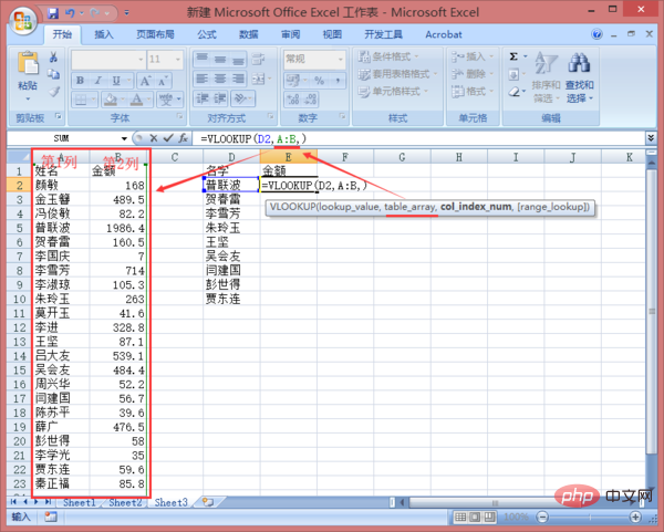
4. Enter the third parameter of the VLOOKUP function: col_index_num. The area contains the column number of the return value, that is, the value to be returned is in the search Column number in the area, because we want to return the value of the amount. As you can see from the picture in step 3, the amount is located in the 2nd column of the search area, so enter: 2, as shown in the figure below.
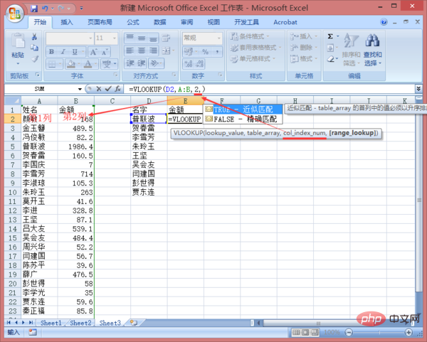
5. Enter the fourth parameter of the VLOOKUP function: range_lookup. If you need an approximate match of the return value, you can specify 1/TRUE; if you need to return For an exact match of values, specify 0/FALSE. Since we want an exact match, enter: 0.
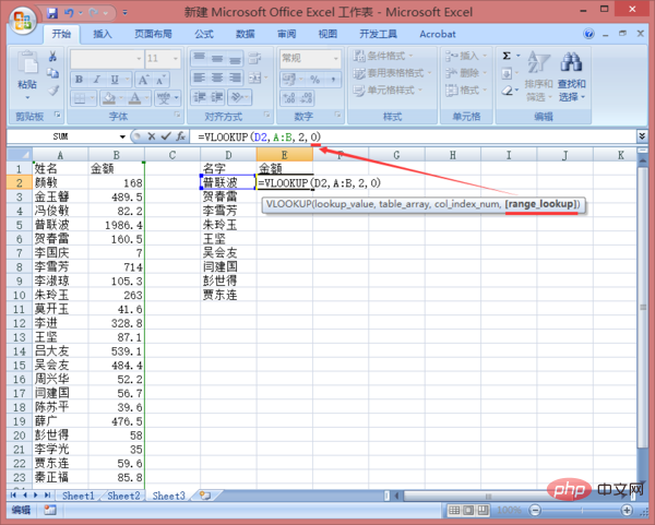
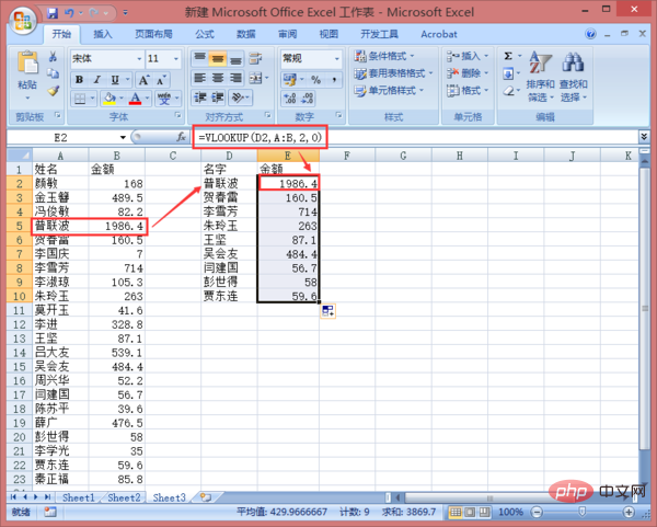
6. Press the Enter key to return to the VLOOKUP function calculation result, and then move the mouse to the lower right corner of cell E2, when it displays the word " " When typing, pull down to copy the formula, and the batch search setting is completed, as shown in the figure below.
The above is the detailed content of How to implement batch matching query in excel. For more information, please follow other related articles on the PHP Chinese website!
 Compare the similarities and differences between two columns of data in excel
 excel duplicate item filter color
 How to copy an Excel table to make it the same size as the original
 Excel table slash divided into two
 Excel diagonal header is divided into two
 Absolute reference input method
 java export excel
 Excel input value is illegal