This article mainly introduces examples of using TensorFlow to implement the Deming regression algorithm. It has a certain reference value. Now I share it with you. Friends in need can refer to it
If the least squares linear regression The algorithm minimizes the vertical distance to the regression line (i.e., parallel to the y-axis direction), then Deming regression minimizes the total distance to the regression line (i.e., perpendicular to the regression line). It minimizes the error in both directions of x value and y value. The specific comparison chart is as follows.
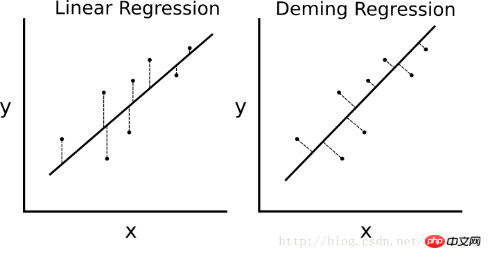
The difference between linear regression algorithm and Deming regression algorithm. The linear regression on the left minimizes the vertical distance to the regression line; the Deming regression on the right minimizes the total distance to the regression line.
The loss function of the linear regression algorithm minimizes the vertical distance; here it is necessary to minimize the total distance. Given the slope and intercept of a straight line, there is a known geometric formula for solving the vertical distance from a point to the straight line. Plug in the geometric formula and have TensorFlow minimize the distance.
The loss function is a geometric formula consisting of a numerator and a denominator. Given a straight line y=mx b and a point (x0, y0), the formula for finding the distance between the two is:

# 戴明回归
#----------------------------------
#
# This function shows how to use TensorFlow to
# solve linear Deming regression.
# y = Ax + b
#
# We will use the iris data, specifically:
# y = Sepal Length
# x = Petal Width

import matplotlib.pyplot as plt
import numpy as np
import tensorflow as tf
from sklearn import datasets
from tensorflow.python.framework import ops
ops.reset_default_graph()

# Create graph
sess = tf.Session()

# Load the data
# iris.data = [(Sepal Length, Sepal Width, Petal Length, Petal Width)]
iris = datasets.load_iris()
x_vals = np.array([x[3] for x in iris.data])
y_vals = np.array([y[0] for y in iris.data])

# Declare batch size
batch_size = 50

# Initialize placeholders
x_data = tf.placeholder(shape=[None, 1], dtype=tf.float32)
y_target = tf.placeholder(shape=[None, 1], dtype=tf.float32)

# Create variables for linear regression
A = tf.Variable(tf.random_normal(shape=[1,1]))
b = tf.Variable(tf.random_normal(shape=[1,1]))

# Declare model operations
model_output = tf.add(tf.matmul(x_data, A), b)

# Declare Demming loss function
demming_numerator = tf.abs(tf.subtract(y_target, tf.add(tf.matmul(x_data, A), b)))
demming_denominator = tf.sqrt(tf.add(tf.square(A),1))
loss = tf.reduce_mean(tf.truep(demming_numerator, demming_denominator))

# Declare optimizer
my_opt = tf.train.GradientDescentOptimizer(0.1)
train_step = my_opt.minimize(loss)

# Initialize variables
init = tf.global_variables_initializer()
sess.run(init)

# Training loop
loss_vec = []
for i in range(250):
  rand_index = np.random.choice(len(x_vals), size=batch_size)
  rand_x = np.transpose([x_vals[rand_index]])
  rand_y = np.transpose([y_vals[rand_index]])
  sess.run(train_step, feed_dict={x_data: rand_x, y_target: rand_y})
  temp_loss = sess.run(loss, feed_dict={x_data: rand_x, y_target: rand_y})
  loss_vec.append(temp_loss)
  if (i+1)%50==0:
    print('Step #' + str(i+1) + ' A = ' + str(sess.run(A)) + ' b = ' + str(sess.run(b)))
    print('Loss = ' + str(temp_loss))

# Get the optimal coefficients
[slope] = sess.run(A)
[y_intercept] = sess.run(b)

# Get best fit line
best_fit = []
for i in x_vals:
 best_fit.append(slope*i+y_intercept)

# Plot the result
plt.plot(x_vals, y_vals, 'o', label='Data Points')
plt.plot(x_vals, best_fit, 'r-', label='Best fit line', linewidth=3)
plt.legend(loc='upper left')
plt.title('Sepal Length vs Pedal Width')
plt.xlabel('Pedal Width')
plt.ylabel('Sepal Length')
plt.show()

# Plot loss over time
plt.plot(loss_vec, 'k-')
plt.title('L2 Loss per Generation')
plt.xlabel('Generation')
plt.ylabel('L2 Loss')
plt.show()Results:
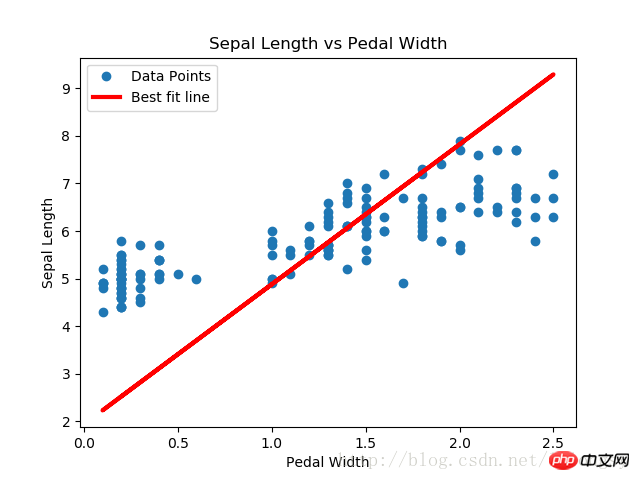
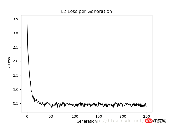
The results obtained by the Deming regression algorithm and linear regression algorithm in this article are basically the same consistent. The key difference between the two is the measurement of the loss function between the predicted value and the data point: the loss function of the linear regression algorithm is the vertical distance loss; while the Deming regression algorithm is the vertical distance loss (total of the x-axis and y-axis). distance loss).
Note that the implementation type of the Deming regression algorithm here is overall regression (total least squares error). The overall regression algorithm assumes that the errors in x and y values are similar. We can also use different errors to expand the distance calculation of the x-axis and y-axis according to different concepts.
Related recommendations:
Sample code for implementing multi-class support vector machines using TensorFlow
TensorFlow implements non-linear support vector machines method
The above is the detailed content of Example of implementing Deming regression algorithm with TensorFlow. For more information, please follow other related articles on the PHP Chinese website!


