This article mainly introduces the detailed explanation of python programming to calculate definite integrals through the Monte Carlo method. It has certain reference value and friends in need can refer to it.
I think back then, when I was taking the postgraduate entrance examination, I wish I had known that there was such a good thing, calculating definite points. . . Just kidding, calculating definite integrals was not that simple at that time. But it did open up an idea for me to use programming languages to solve more complex mathematical problems. Let’s get to the point.

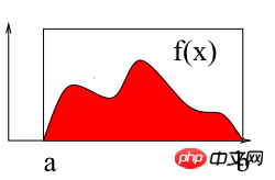
As shown in the figure above, calculating the integral of f(x) on the interval [a b] is to find the area of the red area surrounded by the curve and the X-axis. The following uses the Monte Carlo method to calculate the definite integral on the interval [2 3]: ∫(x2 4*x*sin(x))dx
# -*- coding: utf-8 -*-
import numpy as np
import matplotlib.pyplot as plt

def f(x):
  return x**2 + 4*x*np.sin(x)
def intf(x):
  return x**3/3.0+4.0*np.sin(x) - 4.0*x*np.cos(x)
a = 2;
b = 3;
# use N draws
N= 10000
X = np.random.uniform(low=a, high=b, size=N) # N values uniformly drawn from a to b
Y =f(X)  # CALCULATE THE f(x)
# 蒙特卡洛法计算定积分:面积=宽度*平均高度
Imc= (b-a) * np.sum(Y)/ N;
exactval=intf(b)-intf(a)
print "Monte Carlo estimation=",Imc, "Exact number=", intf(b)-intf(a)
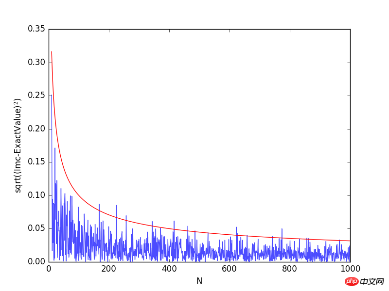
# --How does the accuracy depends on the number of points(samples)? Lets try the same 1-D integral
# The Monte Carlo methods yield approximate answers whose accuracy depends on the number of draws.
Imc=np.zeros(1000)
Na = np.linspace(0,1000,1000)
exactval= intf(b)-intf(a)
for N in np.arange(0,1000):
  X = np.random.uniform(low=a, high=b, size=N) # N values uniformly drawn from a to b
  Y =f(X)  # CALCULATE THE f(x)
  Imc[N]= (b-a) * np.sum(Y)/ N;
plt.plot(Na[10:],np.sqrt((Imc[10:]-exactval)**2), alpha=0.7)
plt.plot(Na[10:], 1/np.sqrt(Na[10:]), 'r')
plt.xlabel("N")
plt.ylabel("sqrt((Imc-ExactValue)$^2$)")
plt.show()


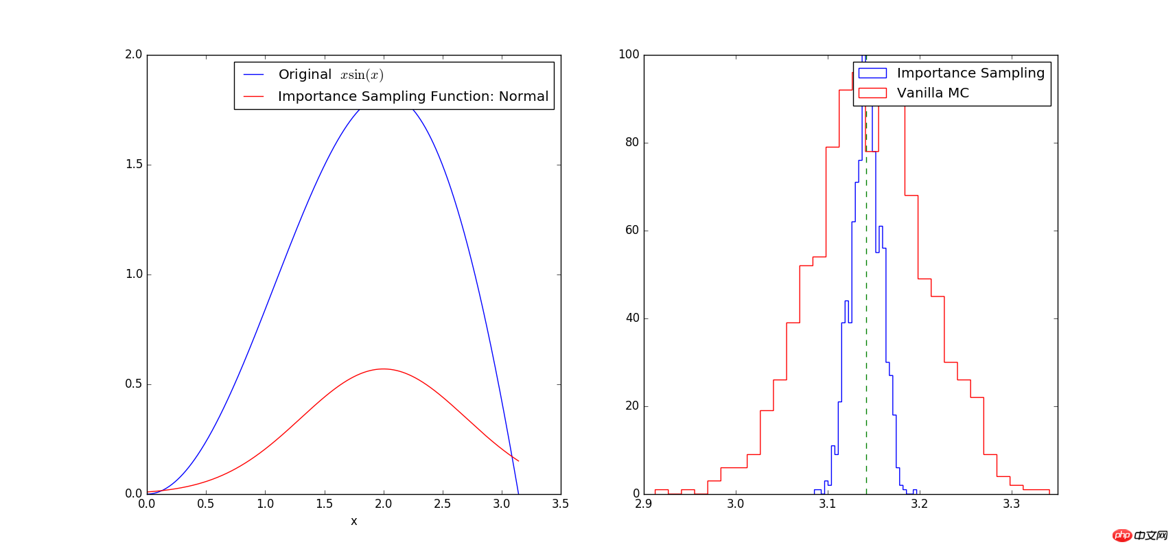
# -*- coding: utf-8 -*- # Example: Calculate ∫sin(x)xdx # The function has a shape that is similar to Gaussian and therefore # we choose here a Gaussian as importance sampling distribution. from scipy import stats from scipy.stats import norm import numpy as np import matplotlib.pyplot as plt mu = 2; sig =.7; f = lambda x: np.sin(x)*x infun = lambda x: np.sin(x)-x*np.cos(x) p = lambda x: (1/np.sqrt(2*np.pi*sig**2))*np.exp(-(x-mu)**2/(2.0*sig**2)) normfun = lambda x: norm.cdf(x-mu, scale=sig) plt.figure(figsize=(18,8)) # set the figure size # range of integration xmax =np.pi xmin =0 # Number of draws N =1000 # Just want to plot the function x=np.linspace(xmin, xmax, 1000) plt.subplot(1,2,1) plt.plot(x, f(x), 'b', label=u'Original $x\sin(x)$') plt.plot(x, p(x), 'r', label=u'Importance Sampling Function: Normal') plt.xlabel('x') plt.legend() # ============================================= # EXACT SOLUTION # ============================================= Iexact = infun(xmax)-infun(xmin) print Iexact # ============================================ # VANILLA MONTE CARLO # ============================================ Ivmc = np.zeros(1000) for k in np.arange(0,1000): x = np.random.uniform(low=xmin, high=xmax, size=N) Ivmc[k] = (xmax-xmin)*np.mean(f(x)) # ============================================ # IMPORTANCE SAMPLING # ============================================ # CHOOSE Gaussian so it similar to the original functions # Importance sampling: choose the random points so that # more points are chosen around the peak, less where the integrand is small. Iis = np.zeros(1000) for k in np.arange(0,1000): # DRAW FROM THE GAUSSIAN: xis~N(mu,sig^2) xis = mu + sig*np.random.randn(N,1); xis = xis[ (xis<xmax) & (xis>xmin)] ; # normalization for gaussian from 0..pi normal = normfun(np.pi)-normfun(0) # 注意:概率密度函数在采样区间[0 pi]上的积分需要等于1 Iis[k] =np.mean(f(xis)/p(xis))*normal # 因此,此处需要乘一个系数即p(x)在[0 pi]上的积分 plt.subplot(1,2,2) plt.hist(Iis,30, histtype='step', label=u'Importance Sampling'); plt.hist(Ivmc, 30, color='r',histtype='step', label=u'Vanilla MC'); plt.vlines(np.pi, 0, 100, color='g', linestyle='dashed') plt.legend() plt.show()
on the interval [0 pi]

How to use NotImplementedError in Python programming_python
The above is the detailed content of Detailed explanation of python programming to calculate definite integrals through Monte Carlo method. For more information, please follow other related articles on the PHP Chinese website!


