This article mainly introduces advanced morphological processing of python digital image processing. Now I will share it with you and give you a reference. Let’s take a look together
Morphological processing, in addition to the most basic expansion, erosion, opening/closing operations, black/white hat processing, there are also some more advanced applications, such as convex hulls and connected region markers , delete small areas, etc.
1. Convex Hull
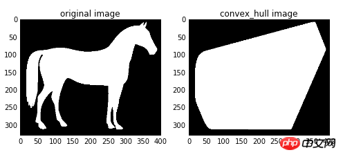
The convex hull refers to a convex polygon that contains all the white pixels in the image.
The function is:
skimage.morphology.convex_hull_image(image)
The input is a binary image and the output is a logical binary image. The points within the convex hull are True, otherwise they are False
Example:
import matplotlib.pyplot as plt from skimage import data,color,morphology #生成二值测试图像 img=color.rgb2gray(data.horse()) img=(img<0.5)*1 chull = morphology.convex_hull_image(img) #绘制轮廓 fig, axes = plt.subplots(1,2,figsize=(8,8)) ax0, ax1= axes.ravel() ax0.imshow(img,plt.cm.gray) ax0.set_title('original image') ax1.imshow(chull,plt.cm.gray) ax1.set_title('convex_hull image')

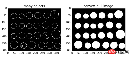
skimage.morphology.convex_hull_object(image,neighbors=8 )
The input parameter image is a binary image, and neighbors indicates whether to use 4-connected or 8-connected. The default is 8-connected. Example:import matplotlib.pyplot as plt from skimage import data,color,morphology,feature #生成二值测试图像 img=color.rgb2gray(data.coins()) #检测canny边缘,得到二值图片 edgs=feature.canny(img, sigma=3, low_threshold=10, high_threshold=50) chull = morphology.convex_hull_object(edgs) #绘制轮廓 fig, axes = plt.subplots(1,2,figsize=(8,8)) ax0, ax1= axes.ravel() ax0.imshow(edgs,plt.cm.gray) ax0.set_title('many objects') ax1.imshow(chull,plt.cm.gray) ax1.set_title('convex_hull image') plt.show()

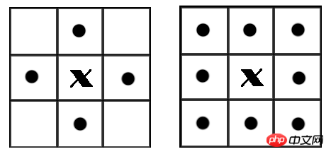
In a binary image, if two pixels are adjacent and have the same value (both 0 or 1), then the two pixels are considered to be in a connected area. All pixels in the same connected area are marked with the same value. This process is called connected area marking. When judging whether two pixels are adjacent, we usually use 4-connected or 8-connected judgment. In an image, the smallest unit is a pixel, and each pixel is surrounded by 8 adjacent pixels. There are two common adjacency relationships: 4-adjacency and 8-adjacency. 4 is adjacent to a total of 4 points, namely up, down, left and right, as shown in the left picture below. 8 There are 8 adjacent points in total, including points at diagonal positions, as shown in the right figure below.
 In the skimage package, we use the label() function under the measure submodule to implement connected area labeling.
Function format:
skimage.measure.label(image,connectivity=None)
The image in the parameter represents the binary image that needs to be processed, connectivity represents the connection mode, 1 represents 4 adjacencies , 2 represents 8 adjacencies.
Output an array of labels (labels), starting from 0.
import numpy as np
import scipy.ndimage as ndi
from skimage import measure,color
import matplotlib.pyplot as plt

#编写一个函数来生成原始二值图像
def microstructure(l=256):
  n = 5
  x, y = np.ogrid[0:l, 0:l] #生成网络
  mask = np.zeros((l, l))
  generator = np.random.RandomState(1) #随机数种子
  points = l * generator.rand(2, n**2)
  mask[(points[0]).astype(np.int), (points[1]).astype(np.int)] = 1
  mask = ndi.gaussian_filter(mask, sigma=l/(4.*n)) #高斯滤波
  return mask > mask.mean()

data = microstructure(l=128)*1 #生成测试图片

labels=measure.label(data,connectivity=2) #8连通区域标记
dst=color.label2rgb(labels) #根据不同的标记显示不同的颜色
print('regions number:',labels.max()+1) #显示连通区域块数(从0开始标记)

fig, (ax1, ax2) = plt.subplots(1, 2, figsize=(8, 4))
ax1.imshow(data, plt.cm.gray, interpolation='nearest')
ax1.axis('off')
ax2.imshow(dst,interpolation='nearest')
ax2.axis('off')

fig.tight_layout()
plt.show()
In the code, by multiplying by 1 in some places, the bool array can be quickly converted to an int array.
The result is as shown in the figure: there are 10 connected areas, marked 0-9
 If you want to operate on each connected area separately, such as calculating Area, circumscribed rectangle, convex hull area, etc., you need to call the regionprops() function of the measure submodule. The format of this function is:
skimage.measure.regionprops(label_image)
Returns the attribute list of all connected blocks. The commonly used attribute list is as follows:
| Type | Description | |
| int | Total number of pixels in the area | ##bbox |
| Boundary bounding box (min_row, min_col, max_row, max_col) | centroid | |
| Centroid coordinates | convex_area | |
| Total number of pixels in the convex hull | convex_image | |
| Convex hull with the same size as the bounding box | coords | |
| Coordinates of pixels in the area | Eccentricity | |
| Eccentricity | equivalent_diameter | |
| The diameter of a circle with the same area as the area | euler_number | |
| Regional Euler number | extent | |
| Regional area and bounding box area Ratio | filled_area | |
| The total number of pixels filled between the area and the bounding box | perimeter | |
| Region perimeter | label | |
| Region label |