


How to Format a Spilled Array in Excel

Use formula conditional formatting to handle overflow arrays in Excel
Direct formatting of overflow arrays in Excel can cause problems, especially when the data shape or size changes. Formula-based conditional formatting rules allow automatic formatting when data parameters change. Adding a dollar sign ($) before a column reference applies a rule to all rows in the data.
In Excel, you can apply direct formatting to the values or background of a cell to make the spreadsheet easier to read. However, when an Excel formula returns a set of values (called overflow arrays), applying direct formatting will cause problems if the size or shape of the data changes.
Suppose you have this spreadsheet with spillover results from the PIVOTBY formula that shows the number of viewers per sport in each region over the past four years.
Since the PIVOTBY function does not contain parameters that allow you to format the results, it is difficult to distinguish between title rows, data rows, subtotal rows, and total rows.
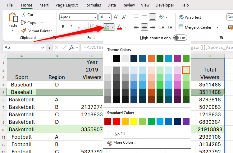
At this point, you might want to apply direct formatting through the Fonts group on the Start tab of the ribbon to intuitively distinguish different types of rows in your data.
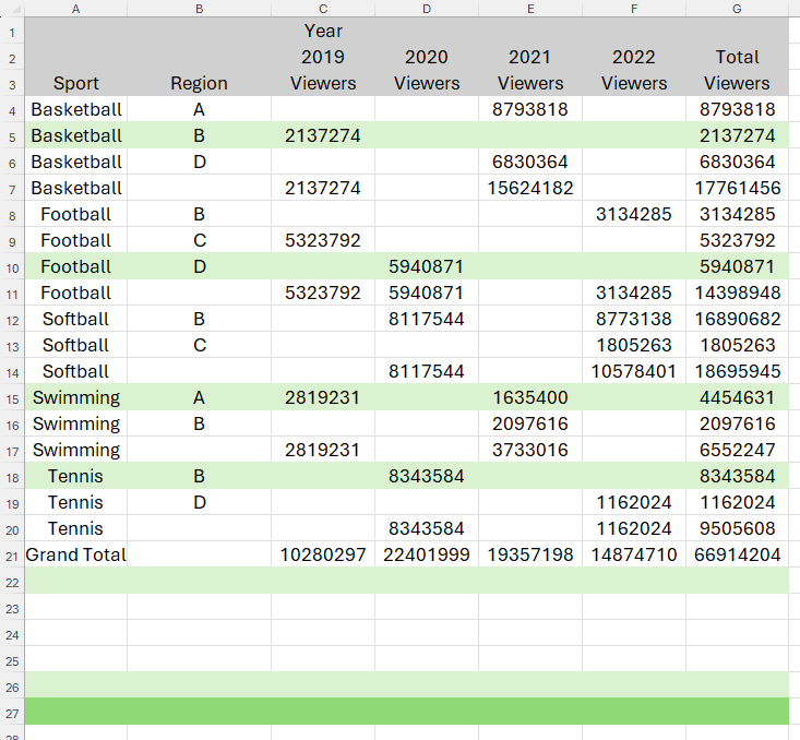
However, if you later modify the parameters in the PIVOTBY formula, or the results are enlarged or reduced due to changes in the original data, the direct formatting you applied will not be adjusted accordingly. This is because direct formatting in Excel is associated with cells, not with the data they contain. See the screenshot below where the data has been reduced, but the direct formatting is still applied to the same row, which can cause confusion.
Instead, you should use conditional formatting, which allows you to format them based on the values of the cells and rows.
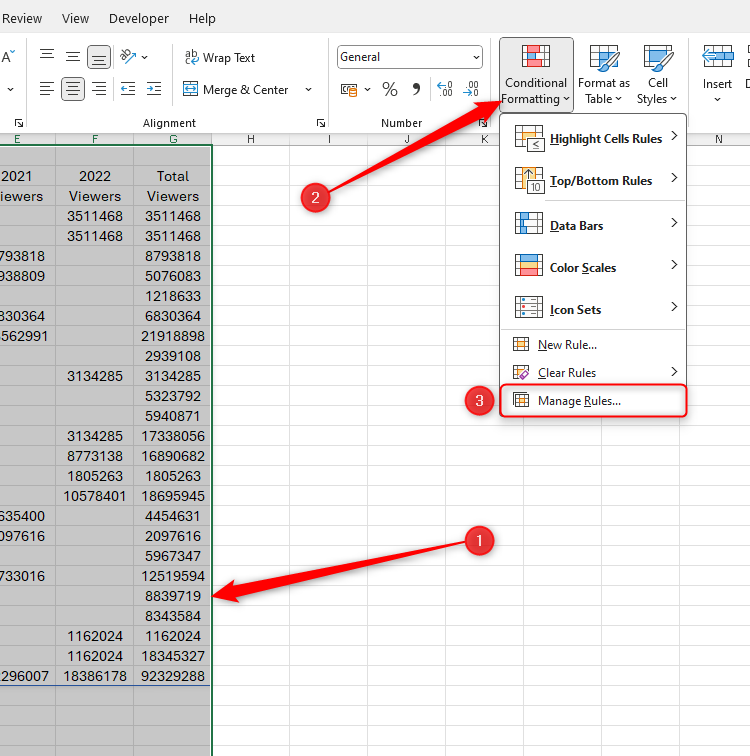
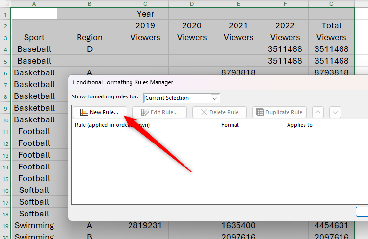
Select all the data (and some extra rows at the bottom to allow vertical growth), and on the Start tab of the ribbon, click Conditional Format > Manage Rules.
Next, in the Conditional Format Rule Manager dialog box, click New Rule.
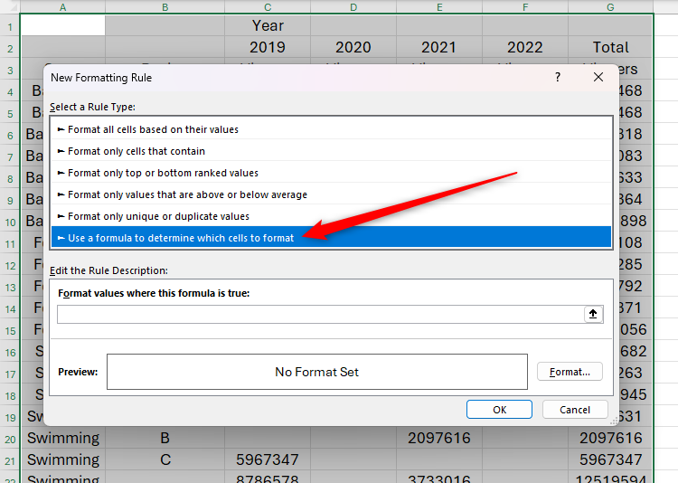
For every rule you will create to format overflow arrays, you need to use formulas. Therefore, in the Select Rule Type area of the New Format Rule dialog box, select the last option Use formula to determine which cell to format.
The first rule you want to create is related to the title line. Specifically, you want these cells to be on a gray background.
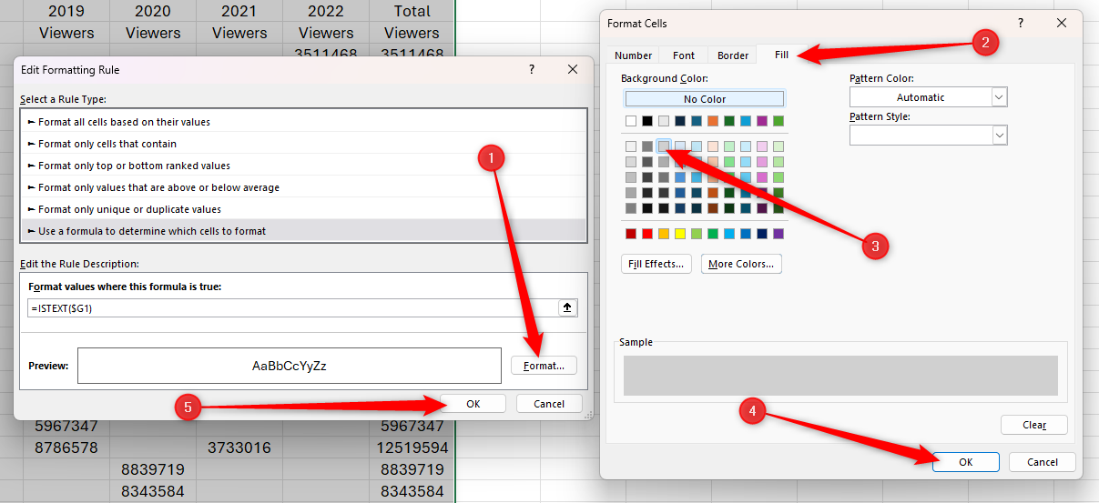
To do this, take a moment to determine what makes the title row different from the other rows in the table. In this example, the title row is the only row in column G that does not contain numbers. So, in the Formula field, type:
<code>=ISTEXT($G1)</code>
Since the ISTEXT function treats empty cells and cells containing text as text values, the conditional formatting rules will consider cells G1 to G3 to contain text, while the rest of the cells in the G column contain numeric values.
Importantly, adding a dollar sign ($) before a column reference repairs the conditional formatting to this column while allowing Excel to apply rules to the rest of the rows.
Finally, because you initially selected the data from columns A to G, the conditional format will be applied to the entire row that satisfies the condition.
Now, click Format to select the format of the title row. In this case, you want them to be gray. Then, click OK in the Format Cell and Edit Format Rules dialog box.
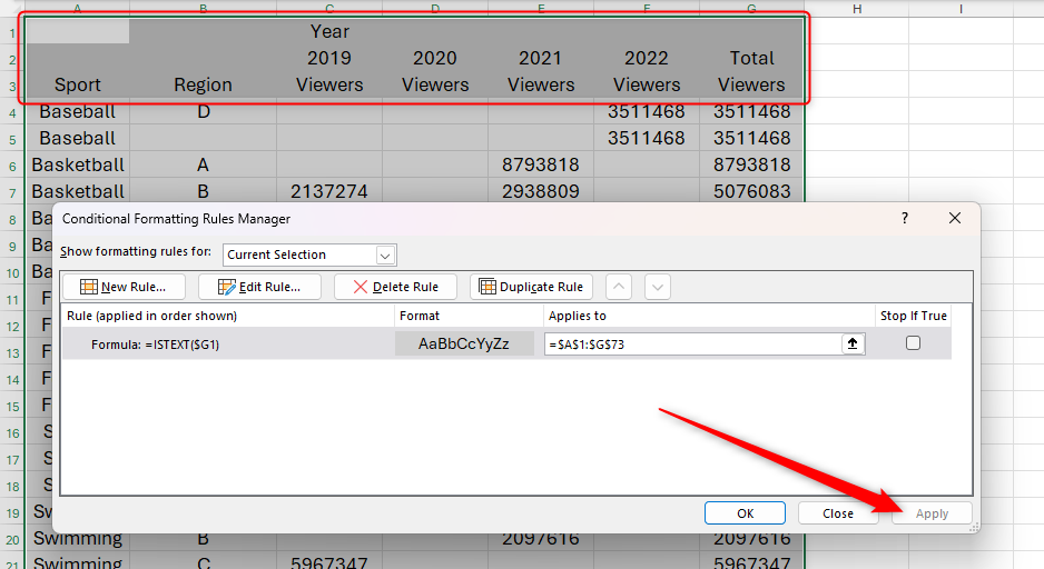
When you click Apply in the Conditional Format Rule Manager dialog box, you will see that only the G columns contain empty cells or text (in other words, the title row) are filled with gray.
Next, you want to format the subtotal rows so they are filled with light green.
Take a closer look at the data again and see which conditions you can use to apply the format to these rows only. In this example, the subtotal row contains text in column A, but nothing in column B. Additionally, since the total row also meets these conditions, you need to exclude any cells in column A that contain the word "total".
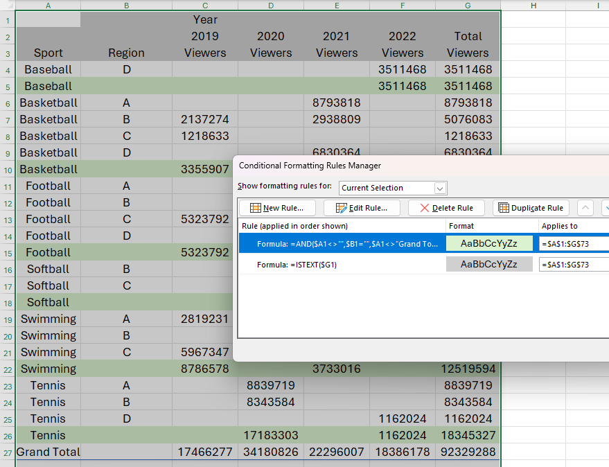
With the Conditional Format Rule Manager dialog box still open, click New Rule and select the option that allows you to format cells using formulas. This time, in the formula field, type:
<code>=AND($A1"",$B1="",$A1"Grand Total")</code>
in:
- The AND function allows you to specify multiple conditions in parentheses.
- $A1" ""Tell Excel to find cells that do not contain () empty cells ("") in column A.
- $B1="" Tell Excel to find cells containing (=) empty cells ("") in column B, and
- $A1"Grand Total" tells Excel to exclude () any cells in column A that contain the text "Grand Total".
As with the previous rules, remember to insert the $ symbol before the column reference to allow Excel to apply the same rule to all selected rows.
Now, click Format to select a light green fill color, and after closing the Format Cells and Edit Format Rules dialog boxes, click Apply to see that the subtotal rows are filled with light green.
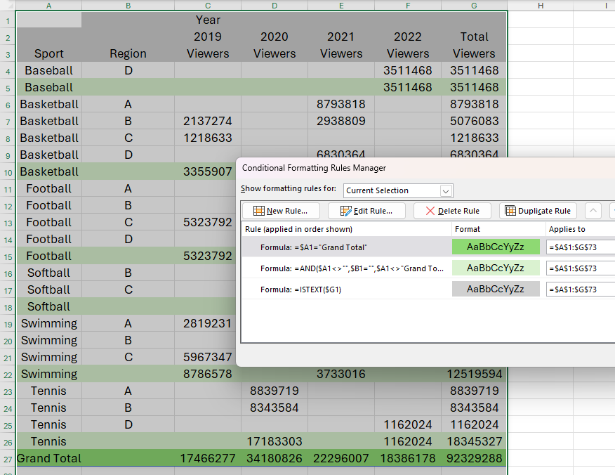
Finally, you want the cells in the total row to be filled with darker green.
Since the total row is the only row in column A that contains the word "total", this is the condition you can use for conditional formatting. In the Conditional Format Rule Manager dialog box, click New Rule, and then select the last option in the Select Rule Type list. Now, in the Formula field, type:
<code>=$A1="Grand Total"</code>
Next, click Format and select the bold green fill color you want to apply to the cell that matches this condition. Now when you close the Format Cells and Edit Format Rules dialogs and click Apply in the Conditional Format Rule Manager dialog, you will see that the total rows are in this format.
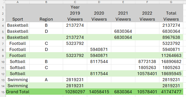
Now that you have applied all the rules, click Close in the Conditional Format Rule Manager dialog box. Then, adjust some data in the original table and see if the overflow results and their formats are updated accordingly.
In this example, even if I delete 12 rows from the original data table, the overflowing PIVOTBY results are still formatted correctly, the title behavior is gray, the subtotal behavior is light green, and the total behavior is bold green.
If you need to change the rules you have created and applied, simply select any cell in the data and click Conditional Format > Manage Rules to restart Conditional Format Rules Manager. Then, double-click the rule to change its conditions.
The above is the detailed content of How to Format a Spilled Array in Excel. For more information, please follow other related articles on the PHP Chinese website!

Hot AI Tools

Undress AI Tool
Undress images for free

Undresser.AI Undress
AI-powered app for creating realistic nude photos

AI Clothes Remover
Online AI tool for removing clothes from photos.

Clothoff.io
AI clothes remover

Video Face Swap
Swap faces in any video effortlessly with our completely free AI face swap tool!

Hot Article
Hot Tools

Notepad++7.3.1
Easy-to-use and free code editor

SublimeText3 Chinese version
Chinese version, very easy to use

Zend Studio 13.0.1
Powerful PHP integrated development environment

Dreamweaver CS6
Visual web development tools

SublimeText3 Mac version
God-level code editing software (SublimeText3)


 How to use the XLOOKUP function in Excel?
Aug 03, 2025 am 04:39 AM
How to use the XLOOKUP function in Excel?
Aug 03, 2025 am 04:39 AM
XLOOKUP is a modern function used in Excel to replace old functions such as VLOOKUP. 1. The basic syntax is XLOOKUP (find value, search array, return array, [value not found], [match pattern], [search pattern]); 2. Accurate search can be realized, such as =XLOOKUP("P002", A2:A4, B2:B4) returns 15.49; 3. Customize the prompt when not found through the fourth parameter, such as "Productnotfound"; 4. Set the matching pattern to 2, and use wildcards to perform fuzzy search, such as "Joh*" to match names starting with Joh; 5. Set the search mode
 how to add page numbers in word
Aug 05, 2025 am 05:51 AM
how to add page numbers in word
Aug 05, 2025 am 05:51 AM
To add page numbers, you need to master several key operations: First, select the page number position and style through the "Insert" menu. If you start from a certain page, you need to insert the "section break" and cancel the "link to the previous section"; second, set the "Home page different" to hide the home page number, check this option in the "Design" tab and manually delete the home page number; third, modify the page number format such as Roman numerals or Arabic numerals, and select and set the starting page number in the "Page Number Format" after sectioning.
 How to add transitions between slides in a PPT?
Aug 11, 2025 pm 03:31 PM
How to add transitions between slides in a PPT?
Aug 11, 2025 pm 03:31 PM
Open the "Switch" tab in PowerPoint to access all switching effects; 2. Select switching effects such as fade in, push, erase, etc. from the library and click Apply to the current slide; 3. You can choose to keep the effect only or click "All Apps" to unify all slides; 4. Adjust the direction through "Effect Options", set the speed of "Duration", and add sound effects to fine control; 5. Click "Preview" to view the actual effect; it is recommended to keep the switching effect concise and consistent, avoid distraction, and ensure that it enhances rather than weakens information communication, and ultimately achieve a smooth transition between slides.
 How to create a photo collage on a single PPT slide?
Aug 03, 2025 am 03:32 AM
How to create a photo collage on a single PPT slide?
Aug 03, 2025 am 03:32 AM
InsertphotosviatheInserttab,resizeandarrangethemusingAligntoolsforneatpositioning.2.Optionally,useatableorshapesasalayoutguidebyfillingcellsorshapeswithimagesforastructuredgrid.3.Enhancevisualsbyapplyingconsistentstyles,effects,andbackgroundoverlaysf
 Complete guide to collaborate in Word and Real Time Co -authorship
Aug 17, 2025 am 01:24 AM
Complete guide to collaborate in Word and Real Time Co -authorship
Aug 17, 2025 am 01:24 AM
Microsoft Word CollolaBate: How to work with co -authors in Word, edit in real time and manage versions easily.
 How to customize the tapes in Office step by step
Aug 22, 2025 am 06:00 AM
How to customize the tapes in Office step by step
Aug 22, 2025 am 06:00 AM
Learn to customize the tapes in Office: Change names, hide chips and create your own commands.
 How AI Will Give Superpowers To ERP Solutions
Aug 29, 2025 am 07:27 AM
How AI Will Give Superpowers To ERP Solutions
Aug 29, 2025 am 07:27 AM
Artificial intelligence holds the key to transforming ERP (Enterprise Resource Planning) systems into next-generation powerhouses—equipping organizations with what can only be described as digital superpowers. This shift isn't just a minor upgrade; i
 How to Create Folders and Files in OneDrive
Aug 03, 2025 am 04:39 AM
How to Create Folders and Files in OneDrive
Aug 03, 2025 am 04:39 AM
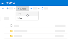
Before you can upload files and folders to OneDrive, it's important to understand how to create them in the first place.Once your files are successfully saved to OneDrive, organizing them effectively can greatly improve your workflow. Below are step-
