How to set percentage filter data in excel_Step tutorial on setting percentage filter data in excel

Data filtering is a commonly used function in Excel, but do you know how to filter percentages? In response to this problem, PHP editor Yuzai will introduce you to the step-by-step tutorial on setting up percentage filtering data in Excel. Through this tutorial, you will learn how to easily filter out data that meets a specific percentage range, helping you quickly locate the key information you need.

1. Open the excel file, select the area where the values need to be filtered, click Start in the ribbon, and find the style toolbar.

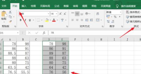
2. In the style toolbar, we can see the conditional formatting tool, click on the bar pattern, and then you can see a series of options.

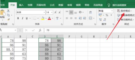
3. As shown in the figure, in the expanded options, we move the mouse to the first/last rule, which is the first and last rule shown in the figure below.

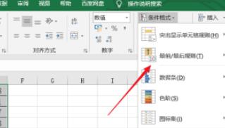
4. As shown in the picture, we can see the following 6 options. Click on the top 10% options pointed by the arrow, and then open the dialog box.

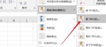
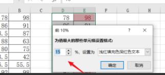
5. In the dialog box below, we can enter the filtering percentage according to our needs, then set the filtering percentage to the color we like, and then click OK.

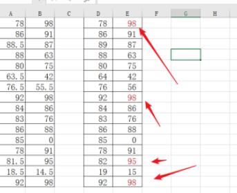
6. After the filtering is completed, return to the Excel page. You can see that the first 15% of the data has been filtered out, and the filtered values are in red font.

The above is the detailed content of How to set percentage filter data in excel_Step tutorial on setting percentage filter data in excel. For more information, please follow other related articles on the PHP Chinese website!