How to use the matching function in office

How to use office matching function

1. Matching keywords--that is, assuming that cell F1 is the matching keyword, enter F1

2. Matching area--to put it simply, you need to find the area that contains the keywords that need to be matched, such as A1:E100

When specifying column extraction, if you need to extract the data in column C from column A where the matching content is located in the area A1:E100, you need to enter the number 3.

4. Exact or fuzzy matching, generally fill in the number 0

for example:

=VLOOKUP(F1,$A$1:$E$100,3,0)

means:

Look for the cell content of F1. Compared with F1, this cell corresponds to the area A1:E100, and extract the content of the cell in column C.

Generally, this function is used to input a number and extract the corresponding content representing this number. For example, if you enter a product number, you can extract the unit price, quantity, and production date of the product number one by one.

How to use VLOOKUP to match data in excel table

In its simplest form, the VLOOKUP function means:

=VLOOKUP (value to look for, range to look for value in, column number in range containing return value, exact match or approximate match – specified as 0/FALSE or 1/TRUE).

Detailed explanation of parameters and key points:

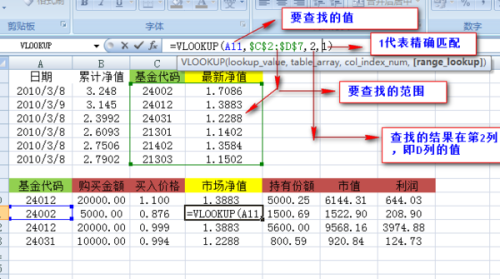
1. The value to be found is also called the lookup value. That is to say, who should be checked according to whom? In the above example it is the "Fund Code".

2. Check the area where the value is located. Remember that the lookup value should always be in the first column of the range for VLOOKUP to work properly. In the above example, it is the area C2:D7.

3. The column number in the area contains the return value. In the above example, the value to be returned is in column D, so C is 1 and D is 2.

(Optional) If an approximate match of the return value is required, you can specify TRUE; if an exact match of the return value is required, specify FALSE. If nothing is specified, the default value will always be TRUE or an approximate match.

How to match the vlookup function in excel

Format:

=VLOOKUP(parameter1,parameter2,parameter3,parameter4)

meaning:

"Parameter 1" is the value that needs to be found in the first column of the array, which can be a numerical value, a reference or a text string; "Parameter 2" is the data table in which the data needs to be found; "Parameter 3" is "Parameter 2" is the column number of the matching value to be returned; "Parameter 4" is a logical value that indicates whether VLOOKUP returns an exact match or an approximate match.

illustrate:

"Parameter 1" is the search content; "Parameter 2" refers to the range of data search (cell area); "Parameter 3" refers to the value to be searched in "Parameter 2", which is the range of data search (cell area) The column number in the area), "Parameter 3" is "2", that is, the value is in the 2nd column. "Parameter 4" is 0 for exact search (can be omitted when it is FALSE).

For example,

"VLOOKUP($F$28,$A$7:$B$1500,2,0)" means to find the row equal to F28 in column A in the range of $A$7:$B$1500 and return to column 2 ( Column B), the last 0 represents exact search;

"VLOOKUP(F28,$A$7:$J$1500,3,0)" means to find the row equal to F28 in column A in the range of $A$7:$J$1500, and return to column 3 (column C ), the last 0 represents exact search.

How Excel automatically matches data

For data returned through multi-condition query matching, it can be achieved through the INDEX MATCH array formula.

The specific operation method is:

1. Open the worksheet of Excel 2007 or above;

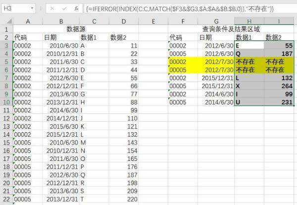
2. Enter the following array formula in the target cell, press the Ctrl Shift Enter key combination to end, and then fill in the formula from the right to the bottom

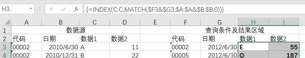
=INDEX(C:C,MATCH($F3&$G3,$A:$A&$B:$B,0))

Formula expression: locate column C and return the data of the row corresponding to the condition that F3 and G3 exist in column A and column B at the same time.

3. When the data area cannot meet the query conditions, an error value #N/A;

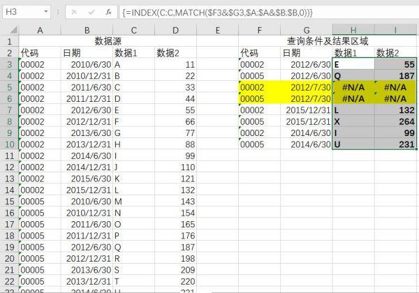
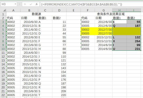
4. You can add the IFERROR function to return the error value as customized content, such as spaces or "does not exist"

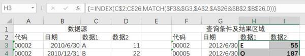
5. If you are using Excel 2003, because Excel 2003 does not support the entire column reference, you need to modify the entire column in the formula to a specific data area. Pay attention to adding the absolute reference symbol $ to avoid referencing when the formula is filled downwards and to the right. The area changes.

The formula is modified to: =INDEX(C$2:C$26,MATCH($F3&$G3,$A$2:$A$26&$B$2:$B$26,0))

6. If you are using Excel 2003, when the data area cannot meet the query conditions, an error value #N/A;

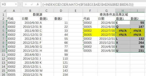
7. Excel 2003 does not support the IFERROR function. You can use the IF ISERROR function instead, and change the formula to

=IF(ISERROR(INDEX(C$2:C$26,MATCH($F3&$G3,$A$2:$A$26&$B$2:$B$26,0))),"＂,INDEX(C $2:C$26,MATCH($F3&$G3,$A$2:$A$26&$B$2:$B$26,0)))

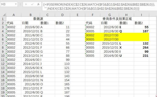
Note: The formulas involved in this column are all array formulas, and you need to press the Ctrl Shift Enter key combination to end, otherwise the error value #N/A will be returned.

The above is the detailed content of How to use the matching function in office. For more information, please follow other related articles on the PHP Chinese website!