


If the execution process of matrix multiplication can be displayed in 3D, it will not be so difficult to learn matrix multiplication back then.
Nowadays, matrix multiplication has become the building block of machine learning models and the basis of various powerful AI technologies. Understanding its execution method will definitely help us understand this AI and this increasingly intelligent system more deeply. world.
This article from the PyTorch blog will introduce mm, a visualization tool for matrix multiplication and matrix multiplication combination.
Because mm uses all three spatial dimensions, compared to ordinary two-dimensional charts, mm helps to intuitively display and stimulate ideas, and uses less cognitive overhead, especially (but not limited to) For people who are good at visual and spatial thinking.
And with three dimensions to combine matrix multiplications, coupled with the ability to load trained weights, mm can visualize large compound expressions (such as attention heads) and observe their actual behavior patterns.
mm is fully interactive, runs in a browser or notebook iframe, and it saves the complete state in the URL, so the link is a shareable session (the screenshots and videos in this article both have a Link, you can open the corresponding visualization in the tool, please refer to the original blog for details). This reference guide describes all available features.
Tool address: https://bhosmer.github.io/mm/ref.html
Original blog text: https://pytorch .org/blog/inside-the-matrix
This article will first introduce the visualization method to build intuition by visualizing some simple matrix multiplications and expressions, and then dive into some extended examples:
Introduction: Why is this visualization better?
Warm-up: Animation - See the working process of standard matrix multiplication decomposition
Warm-up: Expressions - A quick look at some basic expressions Formula building blocks
In-depth attention head: In-depth observation of the structure, value and calculation behavior of a pair of attention heads of GPT-2 through NanoGPT
Parallelize Attention: Visualize parallelization of attention heads using examples from the recent Blockwise Parallel Transformer paper.
Size of attention layer: When we visualize the entire attention layer as a single structure, what do the MHA half and FFA half of the attention layer look like together? How does the image change during the autoregressive decoding process?
LoRA: A visual explanation of the elaboration of this attention head architecture
1 Introduction
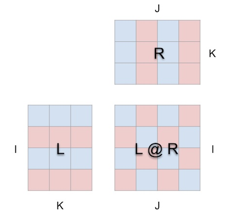
mm's visualization approach is based on the premise that matrix multiplication is essentially a three-dimensional operation.
In other words:
2 Warm-up: Animation
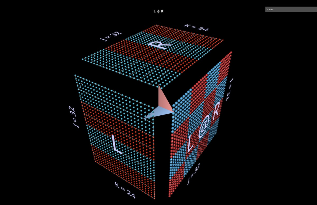
Before we dive into more complex examples, let’s take a look at what this visualization style looks like to establish the Intuitive knowledge of the tool.2a Dot product
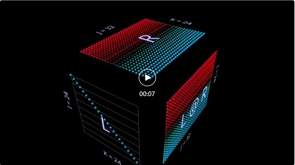
First look at a classic algorithm - calculate each result element by calculating the dot product of the corresponding left row and right column. As you can see from the animation here, the multiplied value vector sweeps through the interior of the cube, each time delivering a summed result at the corresponding location.
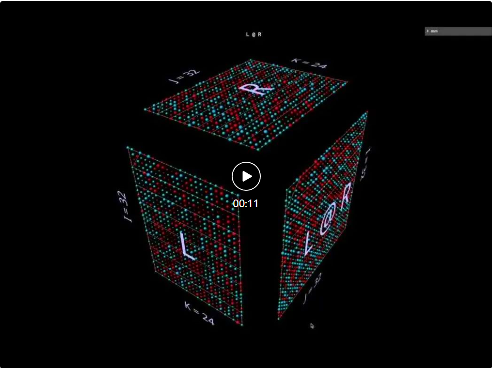
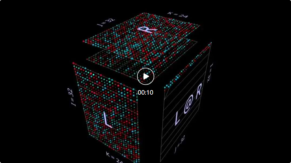
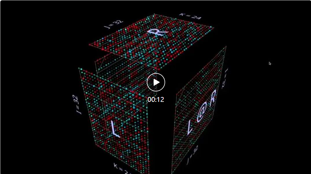
Here, L has blocks of rows filled with 1 (blue) or -1 (red); R has blocks of columns filled similarly. Here k is 24, so the resulting matrix (L @ R) has a blue value of 24 and a red value of -24. 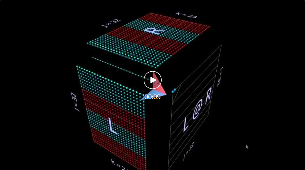
2b Matrix-vector product
Decomposes into matrix-vector product Matrix multiplication looks like a vertical plane (left parameter and the product of each column of the parameter on the right), as it sweeps horizontally across the interior of the cube, plotting the columns onto the result: Interesting, even if the example is simple.  As an example, note that when we use randomly initialized parameters, the middle matrix-vector product highlights the vertical pattern - this reflects the fact that each intermediate value is a column of the left-hand parameter Scaled copy:
Switch to randomly initialized parameters and you can see a matrix-vector product-like pattern -- except this time in horizontal mode, corresponding to the fact that each intermediate vector-matrix product is a row-scaled copy of the right-hand parameter. 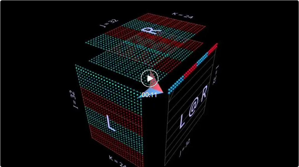 When thinking about how matrix multiplication represents the rank-sum structure of its parameters, it is useful to imagine that both modes occur simultaneously in the calculation:
Here is another An example of using vector-matrix products to build intuition shows that the identity matrix acts like a mirror placed at a 45-degree angle, reflecting its corresponding parameters and results:
The third plane decomposition is to calculate the matrix multiplication result along the k-axis by summing the vector outer products point by point. Here we can see that the outer product plane sweeps the cube "from back to front" and accumulates into the result:
Using a randomly initialized matrix to perform this decomposition, we can not only Looking at the values, you can also see the rank accumulation in the result, as each outer product of rank 1 is added to it. 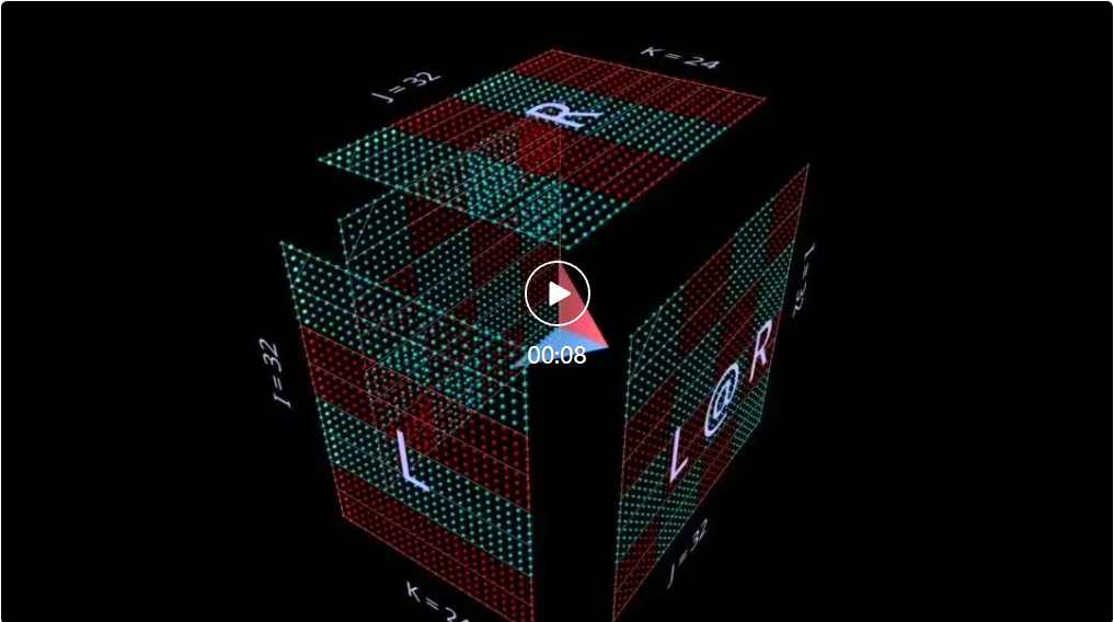 This also intuitively explains why "low-rank factorization" (that is, approximating a matrix by constructing a matrix multiplication with smaller parameters in the depth dimension) works better when the approximated matrix is a low-rank matrix. best effect. This is LoRA that will be mentioned later:
It turns out that this approach scales well for compound expressions. The key rule is simple: the subexpression (sub)matrix multiplication is another cube subject to the same layout constraints as the parent matrix multiplication; the result face of the submatrix multiplication is also the parameter face of the parent matrix multiplication, just like a covalent Shared electrons.
Within these constraints, we can arrange various aspects of submatrix multiplication according to our own needs. The tool's default scheme is used here, which produces alternating convex and concave cubes - this layout works well in practice, maximizing space while minimizing occlusion. (But the layout is fully customizable, see the mm tools page for details.)
This section will visualize some of the key building blocks of machine learning models so that readers can become familiar with this visual representation and gain new intuitions from it. .
3a Left associative expression
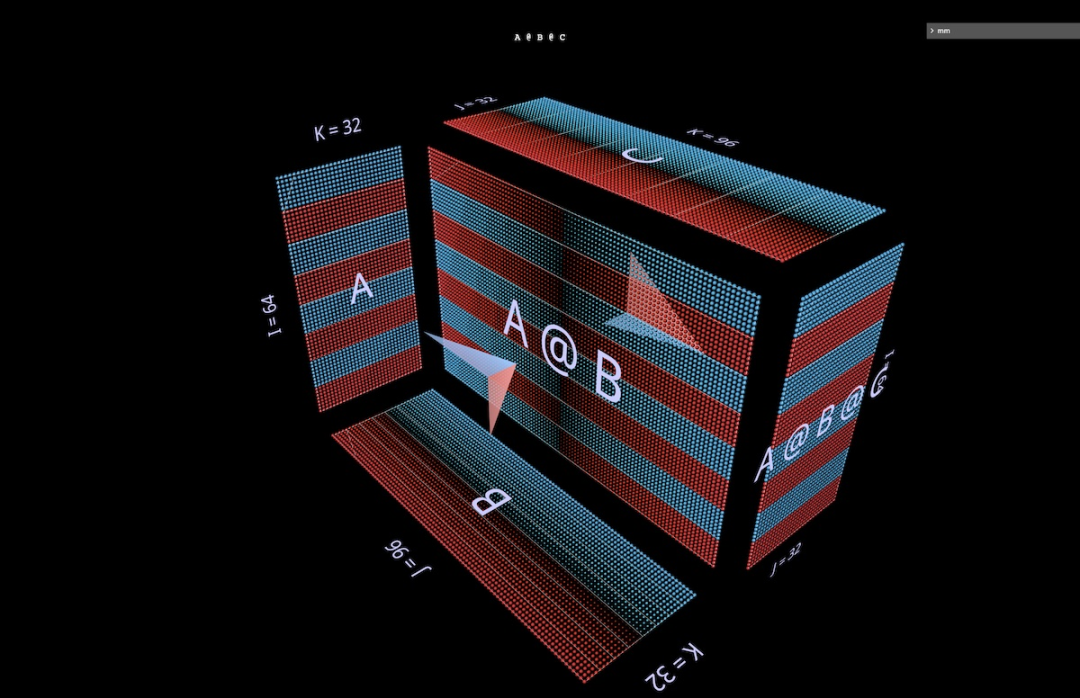
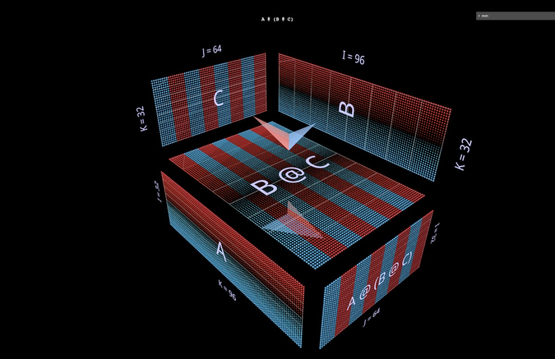
We will introduce two expressions of the form (A @ B) @ C below, each with its own unique shape and feature. (Note: mm follows the convention that matrix multiplication is left associative, so (A @ B) @ C can simply be written as A @ B @ C.)
First give A @ B @ C a very distinctive FFN shape where the "hidden dimension" is wider than the "input" or "output" dimension. (Specifically, for this example, this means that the width of B is greater than the width of A or C.)
Like the single matrix multiplication example, the floating arrow points to the resulting matrix, with the blue fletching From the parameters on the left, the red fletching comes from the parameters on the right.
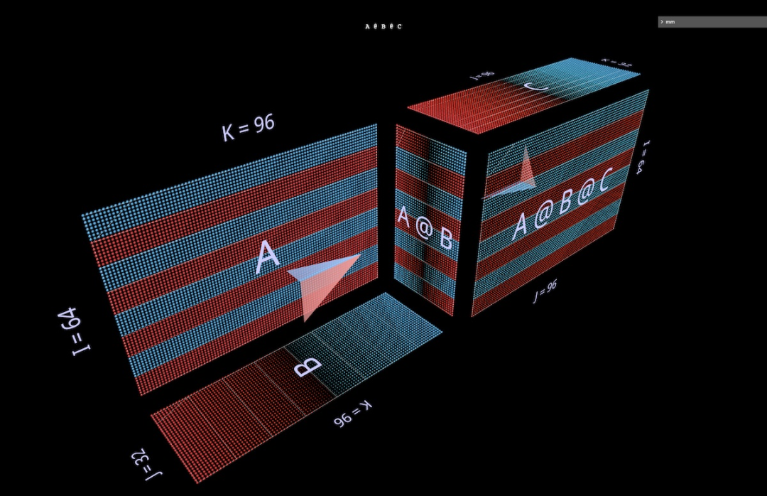
When the width of B is smaller than the width of A or C, there will be a bottleneck in the visualization of A @ B @ C, similar to the shape of an autoencoder.
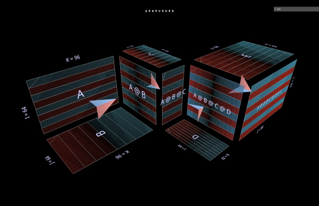
The pattern of alternating bump modules can also be extended to chains of arbitrary lengths: such as this multi-layer bottleneck:
3b Right associative expression
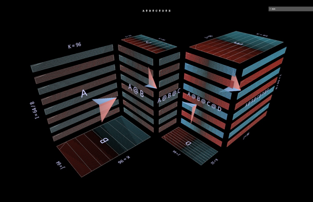
Next, visualize the right associative expression A @ (B @ C).
is similar to the horizontal expansion of the left associative expression - it can be said to start from the left parameter of the root expression, while the right associative expression chain is expanded vertically, starting from the right parameter of the root expression .
One can sometimes see an MLP formed in a right-joining form, where the right-hand side is the columnar input and the weight layer runs from right to left. Using the matrix of the two-layer FFN example depicted above (after appropriate transposition), it would look like this, C is now the input, B is the first layer, and A is the second layer:
Also, in addition to the color of the fletching (blue on the left, red on the right), the second visual cue that distinguishes the left and right parameters is their orientation: the rows of parameters on the left are coplanar with the rows of results — They are stacked along the same axis (i). For example (B @ C) above, both hints can tell us that B is the left-hand parameter.
3c Binary expressions
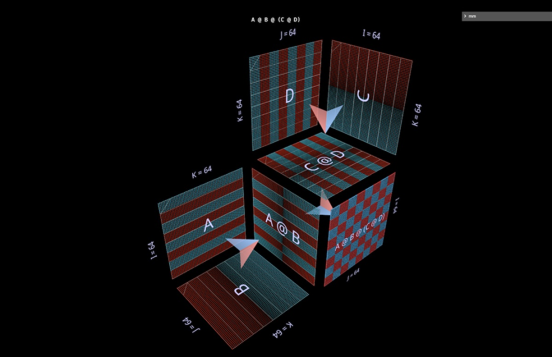
For visualization tools, to be useful, they must not only be used for simple teaching examples, but also be easily used for more complex ones. expression. In real-world use cases, a key structural component is a binary expression - a matrix multiplication with subexpressions on the left and right sides.
The simplest such expression of shape (A @ B) @ (C @ D) is visualized here:
3d A little note: Partitioning and Parallelism
A complete explanation of this topic is beyond the scope of this article, but we will see it in action later in the attention head section. But to warm up, look at two simple examples to see how this style of visualization can make reasoning about parallelized compound expressions very intuitive—just through simple geometric partitioning.
The first example is to apply typical "data parallel" partitioning to the left join multi-layer bottleneck example above. We partition along i, segmenting the initial left-hand parameter (the "batch") and all intermediate results (the "activation"), but not the subsequent parameters (the "weights") - this geometry makes the expression It becomes obvious which actors are segmented and which remain intact:
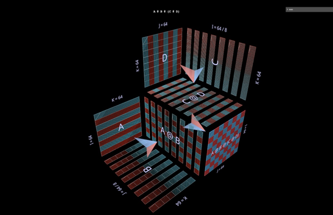
The second example is difficult to understand intuitively without clear geometric support: it shows How to parallelize a binary expression by partitioning the left subexpression along the j axis, the right subexpression along the i axis, and the parent expression along the k axis:
4 Go deep into the head of attention
Now let’s take a look at the attention head of GPT-2 - specifically the "gpt2" (small) configuration of the 4th head of the 5-layer NanoGPT (number of layers = 12, number of heads = 12, number of embeddings = 768), using weights from OpenAI via HuggingFace. Input activations are taken from a forward pass on the OpenWebText training sample containing 256 tokens.
There is nothing special about this particular header, it was chosen mainly because it computes a very common attention pattern and it is located in the middle of the model where activations have become structured and show Some interesting textures.
4a Structure
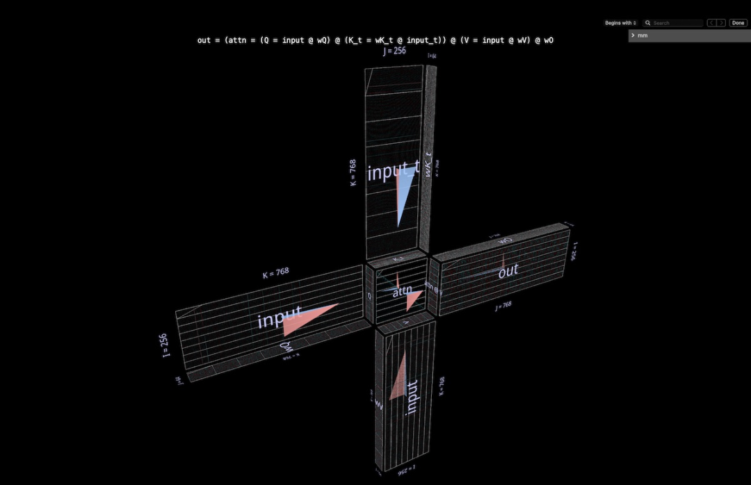
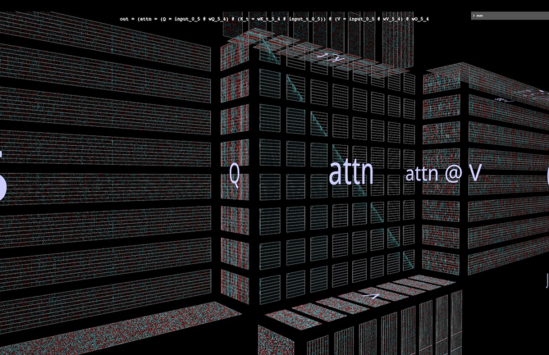
This complete attention head is visualized as a single compound expression, which starts from the input and ends with the projection Output. (Note: To ensure self-sufficiency, output projection is performed for each head as described here for Megatron-LM.)
This calculation involves six matrix multiplications:
Q = input @ wQ// 1K_t = wK_t @ input_t// 2V = input @ wV// 3attn = sdpa(Q @ K_t)// 4head_out = attn @ V // 5out = head_out @ wO // 6
Briefly describe what is being done here:
The blades of the windmill are matrix multiplications 1, 2, 3 and 6: the former group is the inner projection of the input to Q, K and V; The latter is the outer projection from attn@V back to the embedding dimension.
There are two matrix multiplications at the center; the first calculates the attention scores (the convex cube at the back), and then uses them to get the output token based on the value vector (the concave cube at the front) . Causality means that the attention scores form a lower triangle.
But it is better for readers to explore this tool in detail themselves, rather than just looking at screenshots or the video below, in order to understand in more detail - both its structure and the calculation process that flows through it. actual value.
4b Calculating the sum value
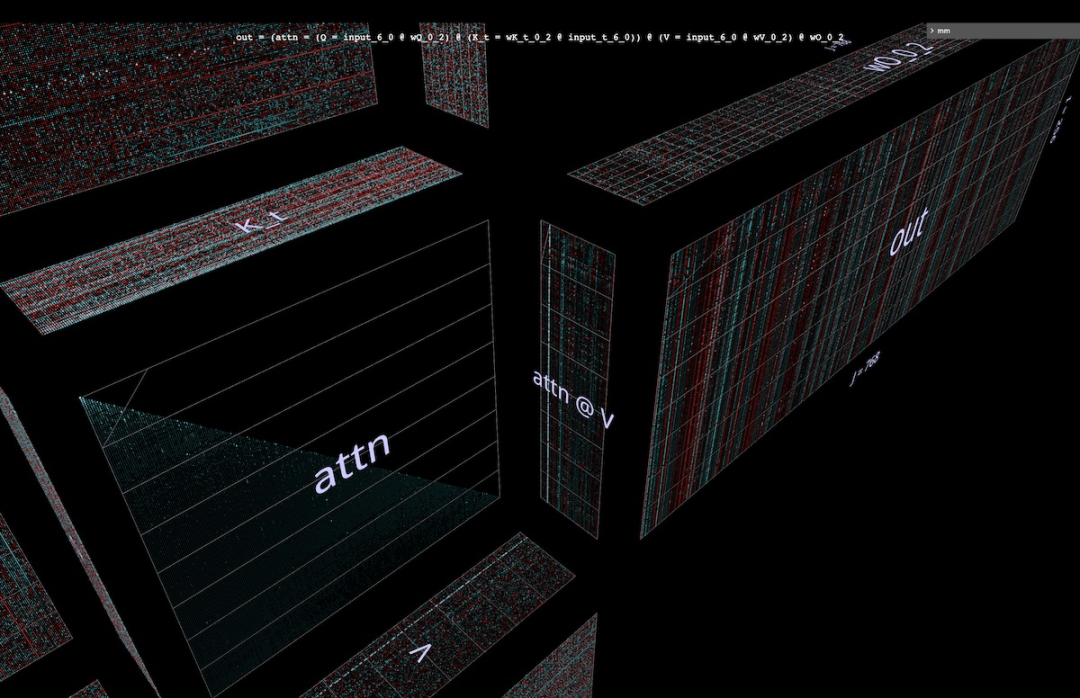
Here is the animation of the calculation process of the attention head. Specifically, we are looking at
sdpa (input @ wQ @ K_t) @ V @ wO
(i.e. matrix multiplications 1, 4, 5 and 6 above, where K_t and V have been pre-computed) as a fusion of vector-matrix products Chains are computed: each item in the sequence passes through attention from input to output in one step. More options for this animation will be covered later in the section on parallelization, but let's first see what the calculated values tell us. 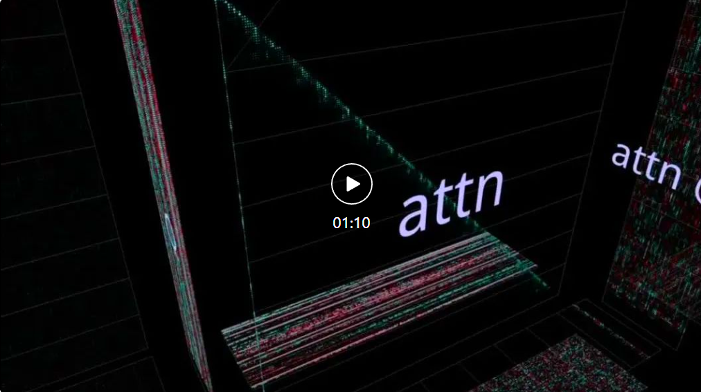
We can see a lot of interesting things:
Before discussing the attention calculation, we can see that the low-rank Q and What an amazing form K_t is in. Zooming in on the Q @ K_t vector-matrix product animation, it looks even more vivid: the large number of channels (embedded positions) in Q and K appear to be more or less constant in the sequence, which means that a useful attention signal may be generated only by A small set of embedded drivers. Understanding and exploiting this phenomenon is part of the SysML ATOM transformer efficiency project.
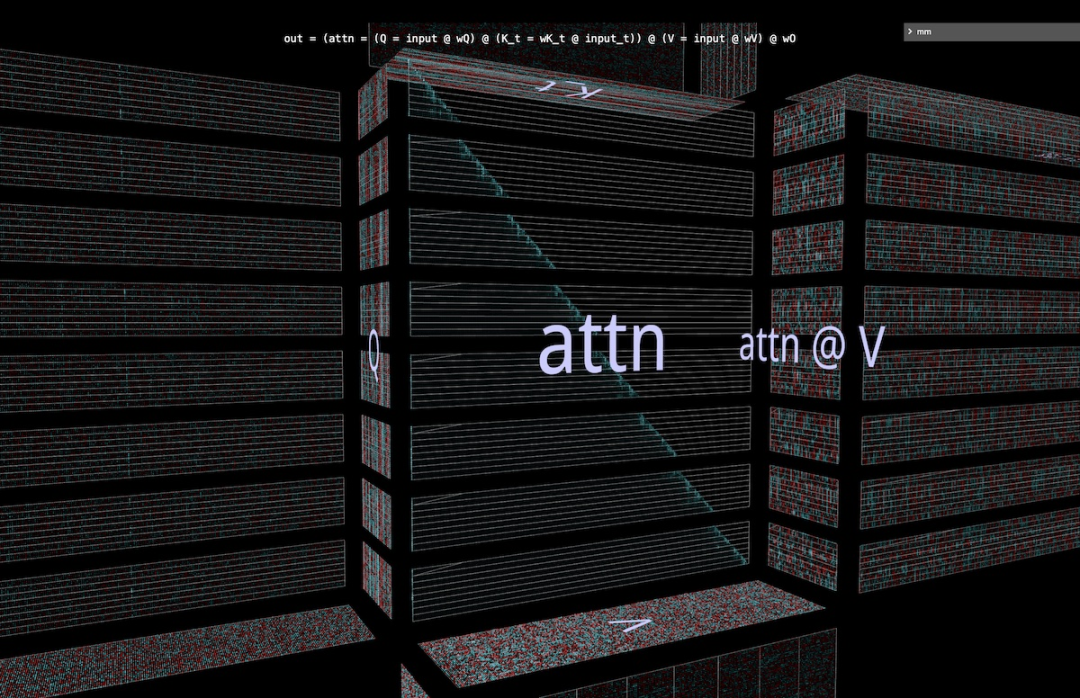
Perhaps the most familiar are the powerful but imperfect diagonals that appear in the attention matrix. This is a common pattern that appears in many attention heads of this model (and many Transformers). It can generate local attention: the value token in the small neighborhood immediately before the output token position largely determines the content pattern of the output token.
However, the size of this neighborhood and the influence of individual tokens within it vary greatly - this can be seen in the off-diagonal frost in the attention grid, and also in The wave pattern seen in the attn[i] @ V vector-matrix product plane as the attention matrix descends along the sequence.
But note that the local neighborhood is not the only thing worth noting: the leftmost column of the attention grid (corresponding to the first token of the sequence) is completely filled with non-zeros (but fluctuating) value, which means that each output token will be affected by the first value token to some extent.
Furthermore, there are imprecise but discernible oscillations in the dominance of attention scores between the current token neighborhood and the initial token. The period of this oscillation varies, but generally it starts out short and then gets longer as you move down the sequence (similarly, given the causality, it is related to the number of candidate attention tokens per row related).
In order to understand how (attn @ V) is formed, it is important not to focus on attention alone - V is equally important. Each output term is a weighted average of the entire V vector: in the extreme case where attention is a perfect diagonal, attn @ V is just an exact copy of V . Here we see something more textured: visible band-like structures where a particular token scores highly on a contiguous subsequence of attention rows, superimposed on a matrix that is clearly similar to V, but with thicker diagonals. There is some vertical occlusion. (Side note: According to the mm reference guide, long-pressing or Control-clicking will display the actual numerical value of the visualization element.)
Keep in mind that since we are in the middle layer (layer 5), the input to this attention head is an intermediate representation, not the original tokenized text. The patterns seen in the input are therefore thought-provoking in their own right - in particular, the strong vertical lines are specific embedding positions whose values uniformly have high amplitude over long stretches of the sequence - sometimes almost full.
But what is interesting is that the first vector in the input sequence is unique, not only breaking the pattern of these high amplitude columns, but also carrying atypical in almost every position value (side note: no visualization here, but this pattern appears repeatedly on multiple sample inputs).
Note: Regarding the last two points, it’s worth reiterating that what is being visualized here is a calculation on a single sample input. In practice, it is found that each head has a characteristic pattern that is consistently (albeit not identically) expressed across a fairly large set of samples, but when looking at any visualization containing activations, one needs to remember that the full distribution of the input may affects in subtle ways the ideas and intuitions it inspires.
Finally, I once again recommend exploring animation directly!
4c There are many interesting differences about attention heads
Before continuing, here is another demonstration showing the usefulness of simply studying the model to understand how it works in detail sex.
This is another attention head of GPT-2. Its behavior pattern is quite different from that of Level 5 Head 4 - as one would expect since it is in a very different part of the model. This header is located on the first layer: Header 2 of layer 0:
Noteworthy points:
Attention to this header The force distribution is very even. This has the effect of delivering the relatively unweighted average of V (or the appropriate causal prefix of V) to each row of attn@V; as shown in the animation: As we move down the attention score triangle, attn[i] @ V vector - matrix product with small fluctuations, rather than simply a scaled-down, gradually revealed copy of V.
attn @ V has amazing vertical uniformity - the same pattern of values persists throughout the sequence in large columnar regions embedded in it. One can think of these as properties shared by each token.
Side note: On the one hand, one might expect attn@V to have some consistency, given the effect of very even distribution of attention. But each row is made up of a causal subsequence of V rather than the entire sequence - why wouldn't this lead to more changes, like a progressive deformation as you move down the sequence? Visual inspection shows that V is not uniform along its length, so the answer must lie in some more subtle property of its value distribution.
Finally, after external projection, the output of this head should be more uniform in the vertical direction.
We can get a strong impression: most of the information conveyed by this attention head consists of attributes shared by each token in the sequence. The composition of its output projection weights can reinforce this intuition.
Overall, we can’t help but wonder: the extremely regular, highly structured information generated by this attention head may have been obtained through slightly... less luxurious computing means. . This is certainly not an unexplored area, but the clarity and richness of visualizing computational signals can be extremely useful for both generating new ideas and reasoning about existing ones.
4d Return to the introduction: free immutability
Looking back, it needs to be reiterated: the reason why we can visualize the non-trivial compound operations of attention and make them Keep it intuitive because important algebraic properties (such as how the shape of a parameter is constrained or which parallel axes intersect which operations) require no additional thinking: they arise directly from the geometric properties of the visualized object, rather than being something extra to remember. rule.
For example, in these attention head visualizations, it can be clearly seen that:
Q has the same length as attn @ V, and K has the same length as V , the lengths of these pairs are independent of each other;
Q has the same width as K, V has the same width as attn @ V, and the widths of these pairs are independent of each other.
These structures are structurally real as a simple result of where in the composite structure the structural components are located and what their orientation is.
The advantage of this "free nature" is particularly useful when exploring variations on typical structures - an obvious example is decoding a single-row high attention matrix in an autoregressive token at a time:

5 Parallelized attention
The animation of head 4 of the 5 layers above visualizes 4 of the 6 matrix multiplications in the attention head .
They are visualized as a fusion chain of vector-matrix products, thus confirming a geometric intuition: the entire left fusion chain from input to output is layered along the shared i-axis and can be parallelized.
5a Example: Partition along i
To parallelize the computation in practice, we can partition the input into blocks along the i axis. We can visualize this partitioning in the tool by specifying that a given axis be divided into a specific number of blocks - 8 will be used in these examples, but there's nothing special about that number.
Besides this, this visualization clearly shows that each parallel computation requires the full wQ (for inner projection), K_t and V (for attention) and wO (for outer projection ) because they are adjacent to partitioned matrices along the unpartitioned dimensions of these matrices:
5b Example: Dual Partitioning
An example of partitioning along multiple axes is also given here. To this end, here we choose to visualize a recent innovation in this field, namely Block Parallel Transformer (BPT), which is based on some research results such as Flash Attention. Please refer to the paper: https://arxiv.org/pdf/2305.19370.pdf
First, BPT partitions along i as described above - and actually extends this horizontal partitioning of the sequence all the way to the other half of the attention layer (FFN). (A visualization of this will be shown later.)
To fully solve this context length problem, add a second partition to MHA - the partition of the attention calculation itself (i.e. along the j-axis of Q@K_t partition). Together, these two partitions divide attention into a grid of blocks:
This is clear from this visualization:
This dual partitioning can effectively solve the context length problem, because we can now visually partition the sequence length of each occurrence in the attention calculation.
The "scope" of the second partition: It is obvious from the geometry that the inner projection calculations of K and V can be partitioned together with the core double matrix multiplication.
Note a subtle detail: the visual hint here is that we can also parallelize the subsequent matrix multiplication attn @ V along k and sum the partial results in split-k style, thereby parallelizing ize the entire double matrix multiplication. But row-by-row softmax in sdpa() adds a requirement: each row has to have all of its segmentation normalized before computing the corresponding row of attn@V, which adds a Additional line-by-line steps.
6 Size of Attention Layer
It is known that the first half of the attention layer (MHA) has a large size due to its quadratic complexity. High computational requirements, but the second half (FFN) also has its own requirements, thanks to the width of its hidden dimension, which is typically 4 times the width of the model's embedding dimension. Visualizing the biomass of a complete attention layer helps build an intuitive understanding of how the two halves of the layer compare to each other.
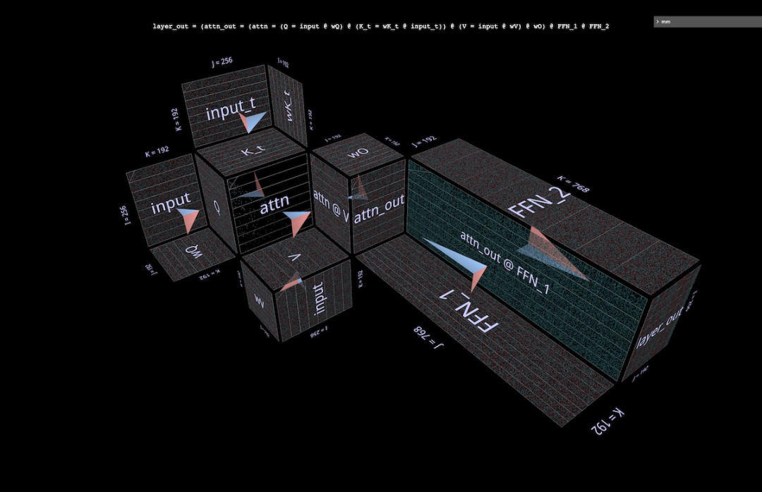
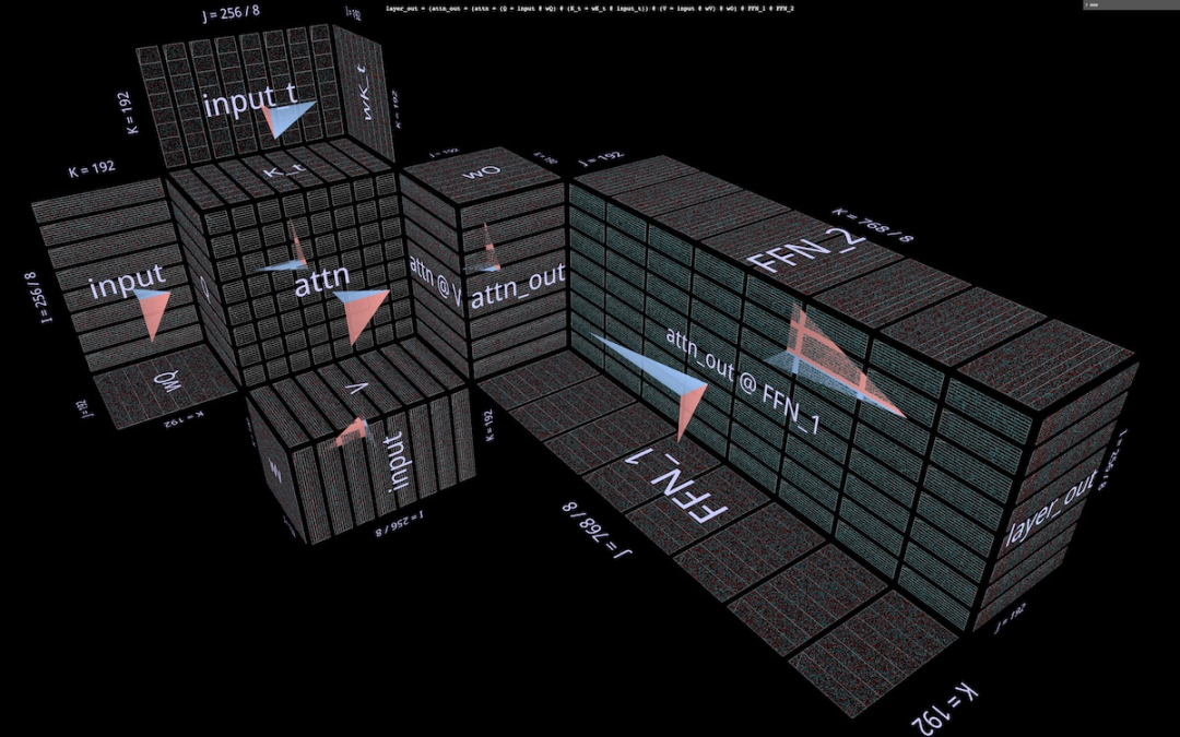
6a Visualizing the complete attention layer
Below is a complete attention layer, with the first half (MHA) at the back and the second half (FFN) at the front. Again, the arrow points in the direction of the calculation.
Note:
This visualization does not depict a single attention head, but shows the unsliced Q/K/V weights and projections around the central double matrix multiplication. Of course this doesn't faithfully visualize the complete MHA operation - but the goal here is to get a clearer idea of the relative matrix sizes in the two halves of the layer, rather than the relative amount of computation performed by each half. (Also, the weights here use random values rather than real weights.)
The dimensions used here are shrunk to ensure that the browser can (relatively) drive them, but the proportions remain the same (small from NanoGPT configuration): model embedding dimension = 192 (originally 768), FFN embedding dimension = 768 (originally 3072), sequence length = 256 (originally 1024), although sequence length has no fundamental impact on the model. (Visually, changes in sequence length will appear as changes in input blade width, resulting in changes in center of attention size and downstream vertical plane height.)
6b Visualizing the BPT Partition Layer
Briefly review the Blockwise Parallel Transformer. Here is a parallelization solution for visualizing BPT in the context of the entire attention layer (each header is omitted as above) . Pay special attention to how the partitioning along i (sequence block) extends through the MHA and FFN halves:
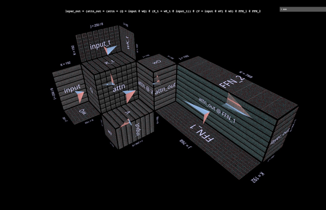
6c Partitioning the FFN
This visualization method suggests an additional partition orthogonal to the one described above - on the FFN half of the attention layer, split the double matrix multiplication (attn_out @ FFN_1) @ FFN_2, first attn_out along j @ FFN_1, then perform subsequent matrix multiplication along k with FFN_2. This partitioning slices the two FFN weight layers to reduce the capacity requirements for each participating component in the calculation, at the expense of the final summation of the partial results.
Here’s what this partitioning method looks like when applied to an unpartitioned attention layer:
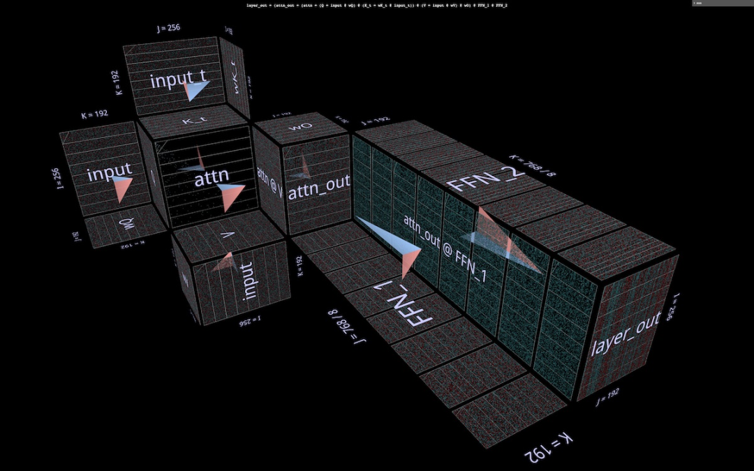
Here’s what it looks like when applied to a BPT-partitioned layer Situation:
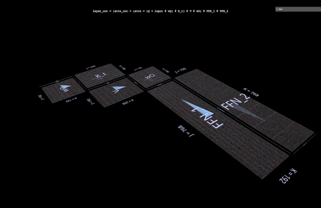
6d Visualize the process of decoding one token at a time
In the autoregressive decoding process of one token at a time , the query vector consists of a single token. It's instructive to imagine in your mind what an attention layer would look like in this case - a single embedding row across a giant tiled plane of weights.
In addition to emphasizing the enormity of weights compared to activations, this view also brings to mind the concept that K_t and V function similarly to dynamically generated layers in a 6-layer MLP, although MHA The mux/demux calculation itself will make this correspondence inaccurate:
7 LoRA
Recent LoRA paper "LoRA : Low-Rank Adaptation of Large Language Models" describes an efficient fine-tuning technique based on the idea that the weight δ introduced during fine-tuning is low-rank. According to the paper, this "allows us to indirectly train some dense layers in a neural network by optimizing the rank decomposition matrix of the dense layer changes during adaptation... while keeping the pre-trained weights frozen."
7a Basic Idea
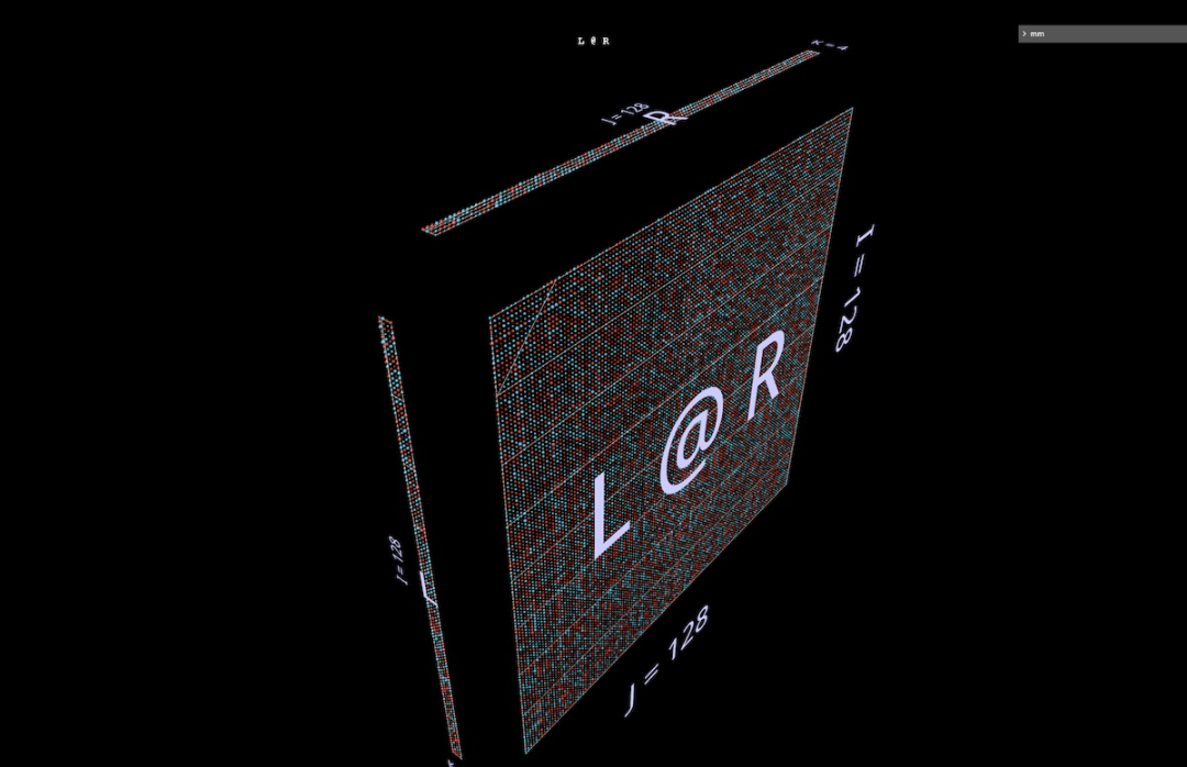
In short, the key step is to train the factors of the weight matrix rather than the matrix itself: matrix multiplication of an I x K tensor and a K x J tensor To replace the I x J weight tensor, it is necessary to ensure that K is a small value.
If K is small enough, there may be a big win in terms of size, but there are trade-offs: reducing K also reduces the rank that the product can express. The size savings and structural impact on the results are illustrated here with an example, here a random matrix multiplication of 128 x 4 left-hand parameters and 4 x 128 right-hand parameters - that is, a 128 x 128 matrix with rank 4 break down. Note the vertical and horizontal modes in L@R:
#7b Apply LoRA to the attention head
LoRA applies this The way the decomposition method is applied to the fine-tuning process is:
Create a low-rank decomposition for each weight tensor to be fine-tuned, and train its factors while keeping the original weights frozen;
After fine-tuning, multiply each pair of low-rank factors to get a matrix in the shape of the original weight tensor and add it to the original pre-trained weight tensor.
The visualization below shows an attention head with its weight tensors wQ, wK_t, wV, wO replaced by low-rank decompositions wQ_A @ wQ_B, etc. Visually, the factor matrix appears as a low fence along the edge of a windmill blade: 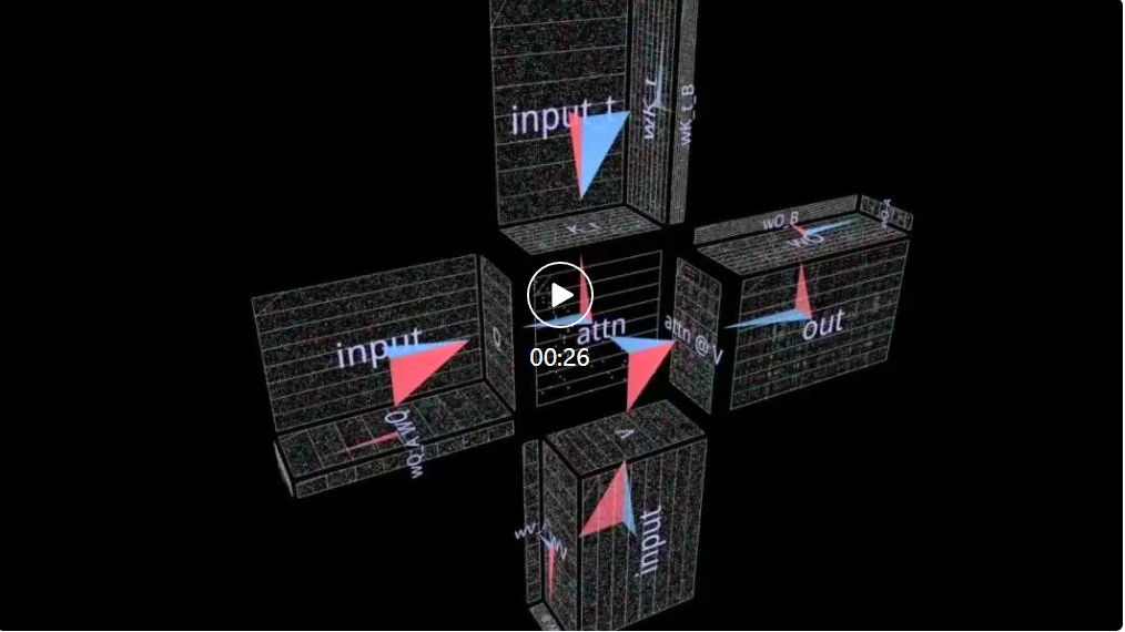
The above is the detailed content of Insight into matrix multiplication from a 3D perspective, this is what AI thinking looks like. For more information, please follow other related articles on the PHP Chinese website!


![[Web front-end] Node.js quick start](https://img.php.cn/upload/course/000/000/067/662b5d34ba7c0227.png)


