Regression analysis and best fit straight line using Python

In this tutorial, we will use Python programming to implement regression analysis and best-fit lines

Introduction

Regression analysis is the most basic form of predictive analysis.

In statistics, linear regression is a method of modeling the relationship between a scalar value and one or more explanatory variables.

In machine learning, linear regression is a supervised algorithm. This algorithm predicts a target value based on independent variables.

More information about linear regression and regression analysis

In linear regression/analysis, the target is a real or continuous value such as salary, BMI, etc. It is often used to predict the relationship between a dependent variable and a set of independent variables. These models typically fit linear equations, however, there are other types of regression, including higher-order polynomials.

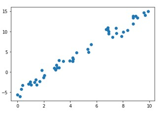
Before fitting a linear model to the data, it is necessary to check whether there is a linear relationship between the data points. This is evident from their scatter plot. The goal of the algorithm/model is to find the line of best fit.

In this article, we will explore linear regression analysis and its implementation using C.

The form of the linear regression equation is Y = c mx, where Y is the target variable and X is the independent variable or explanatory parameter/variable. m is the slope of the regression line and c is the intercept. Since this is a 2D regression task, the model tries to find the line of best fit during training. All points don't have to line up exactly on the same line. Some data points may lie on the line, and some may be scattered across the line. The vertical distance between the line and the data points is the residual. The value can be negative or positive depending on whether the point is below or above the line. The residual is a measure of how well the line fits the data. The algorithm is continuous to minimize the total residual.

The residual for each observation is the difference between the predicted value of y (the dependent variable) and the observed value of y

$$\mathrm{residual\: =\:actual\:y\:value\:−\:forecast\:y\:value}$$

$$\mathrm{ri\:=\:yi\:−\:y'i}$$

The most common metric for evaluating the performance of a linear regression model is called the root mean square error, or RMSE. The basic idea is to measure how bad/wrong the model's predictions are compared to actual observations.

Therefore, high RMSE is "bad" and low RMSE is "good"

RMSE error is

$$\mathrm{RMSE\:=\:\sqrt{\frac{\sum_i^n=1\:(this\:-\:this')^2}{n}}}$$ p>

RMSE is the root of the mean square of all residuals.

Using Python to implement

Example

# Import the libraries
import numpy as np
import math
import matplotlib.pyplot as plt
from sklearn.linear_model import LinearRegression
from sklearn.metrics import mean_squared_error

# Generate random data with numpy, and plot it with matplotlib:
ranstate = np.random.RandomState(1)
x = 10 * ranstate.rand(100)
y = 2 * x - 5 + ranstate.randn(100)
plt.scatter(x, y);
plt.show()

# Creating a linear regression model based on the positioning of the data and Intercepting, and predicting a Best Fit:
lr_model = LinearRegression(fit_intercept=True)
lr_model.fit(x[:70, np.newaxis], y[:70])
y_fit = lr_model.predict(x[70:, np.newaxis])

mse = mean_squared_error(y[70:], y_fit)
rmse = math.sqrt(mse)

print("Mean Square Error : ",mse)
print("Root Mean Square Error : ",rmse)

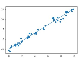
# Plot the estimated linear regression line using matplotlib:
plt.scatter(x, y)
plt.plot(x[70:], y_fit);
plt.show()

Output

Mean Square Error : 1.0859922470998231 Root Mean Square Error : 1.0421095178050257

in conclusion

Regression analysis is a very simple yet powerful technique used for predictive analysis in machine learning and statistics. The idea lies in its simplicity and the underlying linear relationship between the independent and target variables.

The above is the detailed content of Regression analysis and best fit straight line using Python. For more information, please follow other related articles on the PHP Chinese website!