How to use large visual models to accelerate training and inference?

Hello everyone, I am Tao Li from the NVIDIA GPU computing expert team. I am very happy to have the opportunity to share with you today what my colleague Chen Yu and I have done in the Swin Transformer visual model. Some work on type training and inference optimization. Some of these methods and strategies can be used in other model training and inference optimization to improve model throughput, improve GPU usage efficiency, and speed up model iteration.

I will introduce the optimization of the training part of the Swin Transformer model. The work on the inference optimization part will be introduced in detail by my colleagues

Here is the directory we shared today, which is mainly divided into four parts. Since it is optimized for a specific model, let’s first I will briefly introduce the Swin Transformer model. Then, I will combine the profiling tool, that is, nsight system, to analyze and optimize the training process. In the inference part, my colleagues will give strategies and methods for inference optimization, including more detailed CUDA-level optimization. Finally, here is a summary of today’s optimization content.

First is the first part, which is the introduction of Swin Transformer.

1. Introduction to Swin Transformer

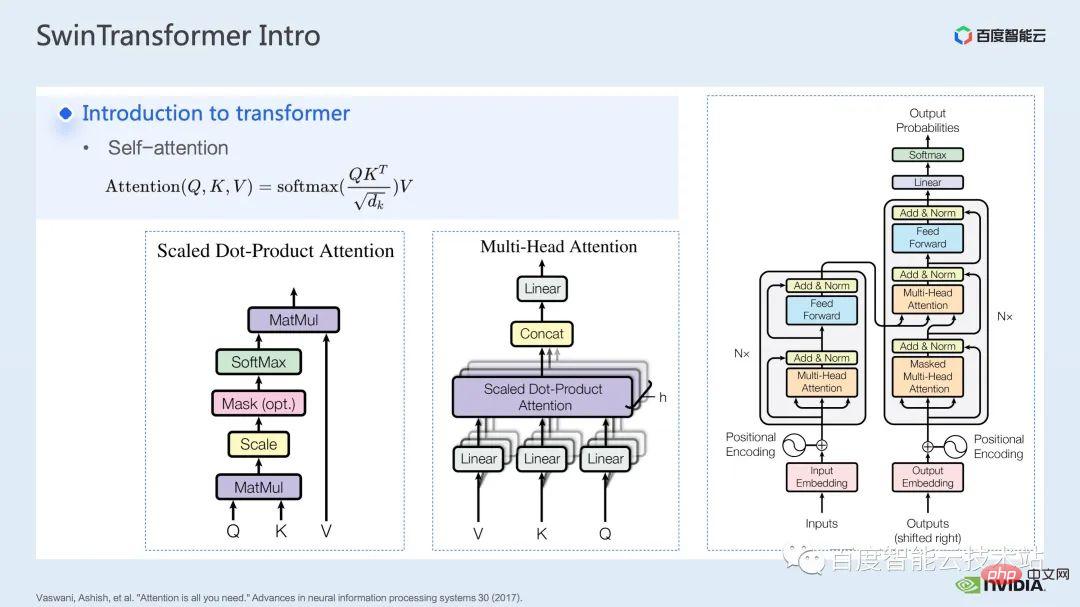
We can see from the name of the model, This is a model based on transformer. Let's briefly review the transformer first.

After the Transformer model was proposed in the article attention is all you need, it has shined on many tasks in the field of natural language processing.

The core of the Transformer model is the so-called attention mechanism, which is the attention mechanism. For the attention module, the usual inputs are query, key and value tensors. Through the function of query and key, plus the calculation of softmax, the attention result usually called attention map can be obtained. According to the value in the attention map, the model can learn which areas in the value need to pay more attention to, or It is said that the model can learn which values in value are of great help to our task. This is the most basic single-head attention model.

We can form a common multi-head attention module by increasing the number of such single-head attention modules. Common encoders and decoders are built based on such multi-head attention modules.

Many models usually include two types of attention modules: self-attention and cross-attention, or a stack of one or more modules. For example, the famous BERT is composed of multiple encoder modules. The popular diffusion model usually includes both self-attention and cross-attention.

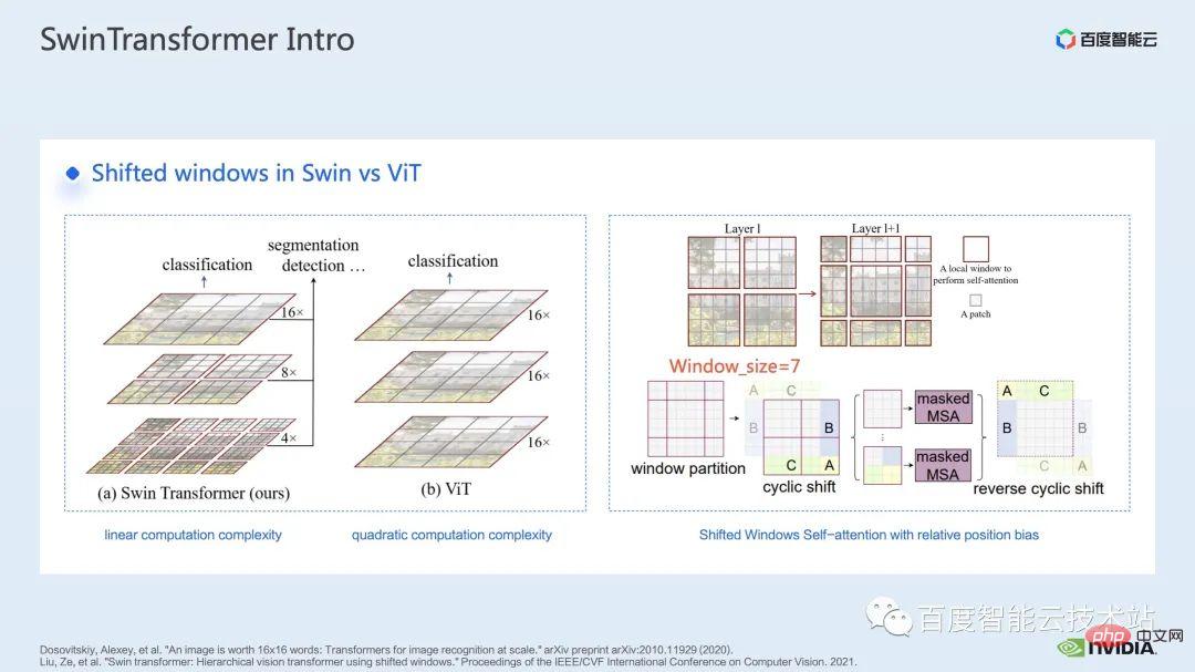
Before Swin Transformer, Vision Transformer (ViT) first applied transformers to the field of computer vision. The model structure of ViT is shown on the left side of the figure below. ViT will divide an image into a series of patches. Each patch is analogous to a token in natural language processing, and then encodes this series of patches through a Transformer-based encoder. , and finally obtain features that can be used for tasks such as classification.

Coming to Swin Transformer, it introduces the concept of window attention. Unlike ViT, which pays attention to the entire image, Swin Transformer will first divide the image into several window, and then only pay attention to the patches inside the window, thereby reducing the amount of calculation.

In order to make up for the boundary problem caused by window, Swin Transformer further introduces the window shift operation. At the same time, in order to make the model have richer position information, relative position bias is also introduced in attention. In fact, the window attention and window shift here are the origin of the name Swin in Swin Transformer.

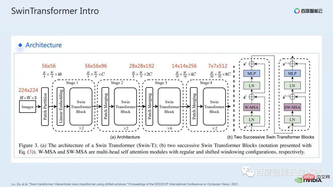
What is given here is the network structure of Swin Transformer. A rough network structure is very similar to traditional CNN such as ResNet. similar.

It can be seen that the entire network structure is divided into multiple stages. In the middle of different stages, there will be a corresponding downsampling process. The resolution of each stage is different, thus forming a resolution pyramid, which also gradually reduces the computational complexity of each stage.

# Then there will be several transformer blocks in each stage. In each transformer block, the window attention module mentioned above will be used.

Next, we will deconstruct Swin Transformer from the perspective of specific operations.

As you can see, a transformer block involves three parts. The first part is the window-related operations of window shift/partition/reverse, and the second part is the attention calculation, and the third part is the FFN calculation; the attention and FFN parts can be further subdivided into several ops, and finally we can subdivide the entire model into a combination of dozens of ops.

# Such operator division is very important for us to conduct performance analysis, locate performance bottlenecks and carry out acceleration optimization.

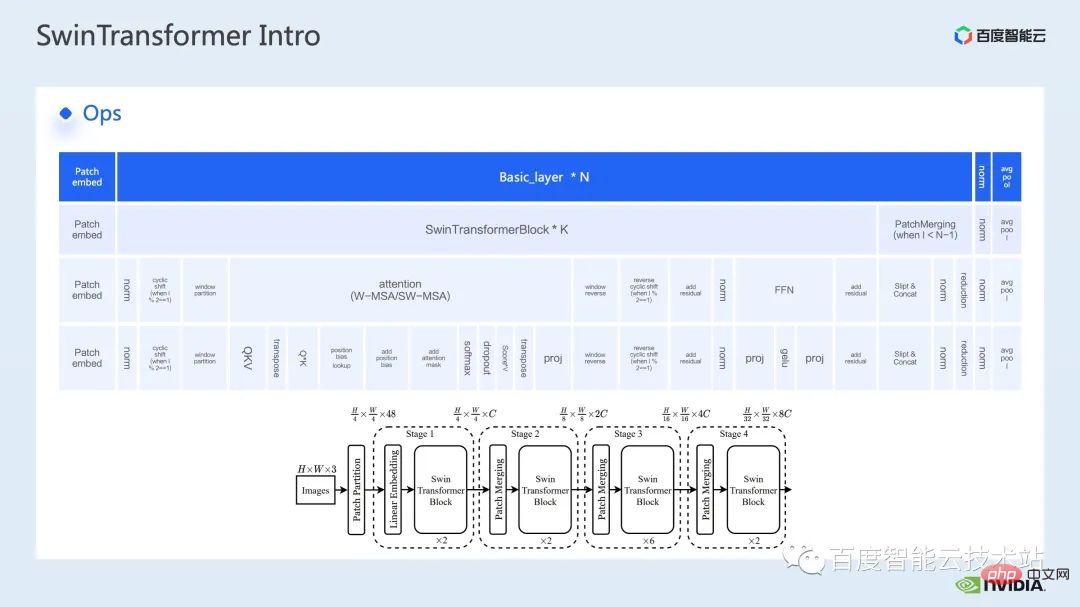
The above is the introduction to the first part. Next, let’s introduce some of the optimization work we have done in training. In particular, we combine the profiling tool, namely nsight system, to analyze and optimize the overall training process.

2. Swin Transformer training optimization

For large For model training, multi-card and multi-node computing resources are usually used. For Swin Transformer, we found that the overhead of inter-card communication will be relatively small. As the number of cards increases, the overall speed increases almost linearly, so here, we give priority to analyzing the computing bottlenecks on a single GPU. and optimization.

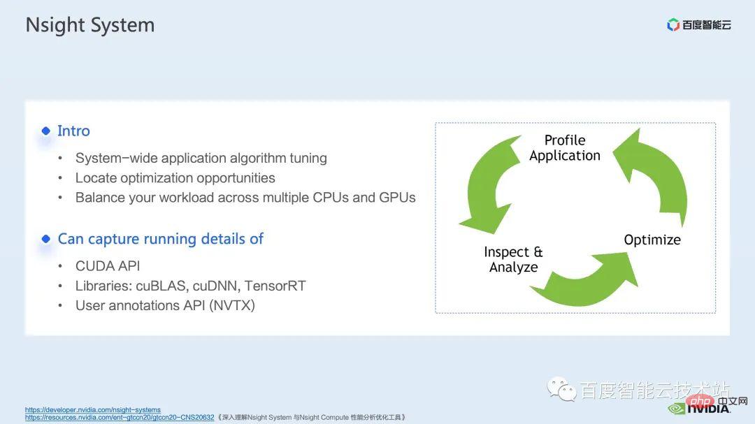
nsight system is a system-level performance analysis tool. Through this tool, we can easily see the GPU usage of each module of the model. Whether there are possible performance bottlenecks and optimization space such as data waiting can make it easier for us to reasonably plan the load between the CPU and GPU.

nsight system can capture the calling and running status of kernel functions called by CUDA and some gpu computing libraries such as cublas, cudnn, tensorRT, etc. And it is convenient for users to add some marks to count the operation of the corresponding gpu within the mark range.

A standard model optimization process is shown in the figure below. We profile the model, get the performance analysis report, discover performance optimization points, and then target them to do performance tuning.

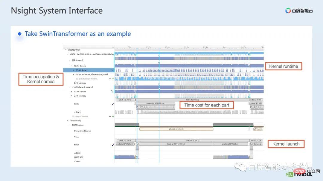
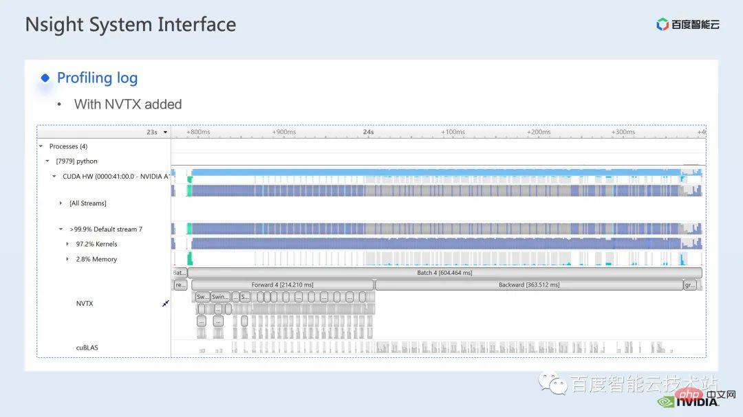
This is an interface of nsight system. We can clearly see the launch of the kernel function, which is the kernel launch; the running of the kernel function, which is the runtime part here. For specific kernel functions, we can see the time proportion in the entire process, and whether the GPU is idle and other information. After adding the nvtx tag, we can see the time it takes for the model to move forward and reverse.

In the forward part, if we zoom in, we can also clearly see the specific calculation needs of each SwinTransformer Block time.

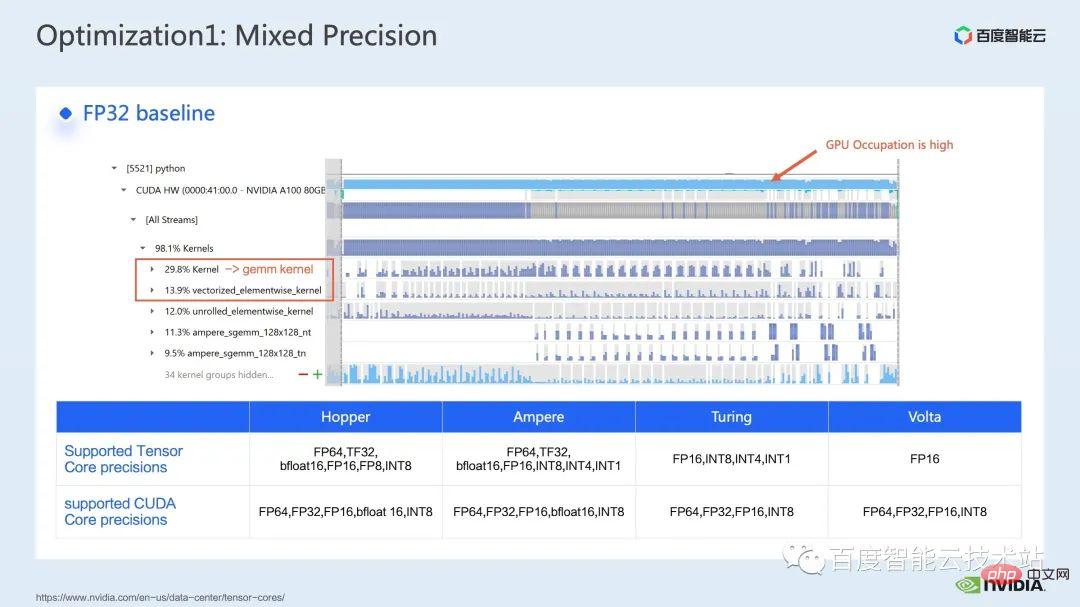
We first use the nsight system performance analysis tool to look at the performance of the entire baseline, as shown in the figure below From the baseline of FP32, we can see that its GPU utilization is very high, and the highest proportion is the matrix multiplication kernel.

#So for matrix multiplication, one of our optimization methods is to make full use of tensor core for acceleration.

We know that NVIDIA’s GPU has hardware resources such as cuda core and tensor core. Tensor core is a module specifically designed to accelerate matrix multiplication. We can consider using tf32 tensor core directly or using fp16 tensor core in mixed precision. You should know that the throughput of matrix multiplication of tensor core using fp16 will be higher than that of tf32, and the matrix multiplication of pure fp32 will also have a high acceleration effect.

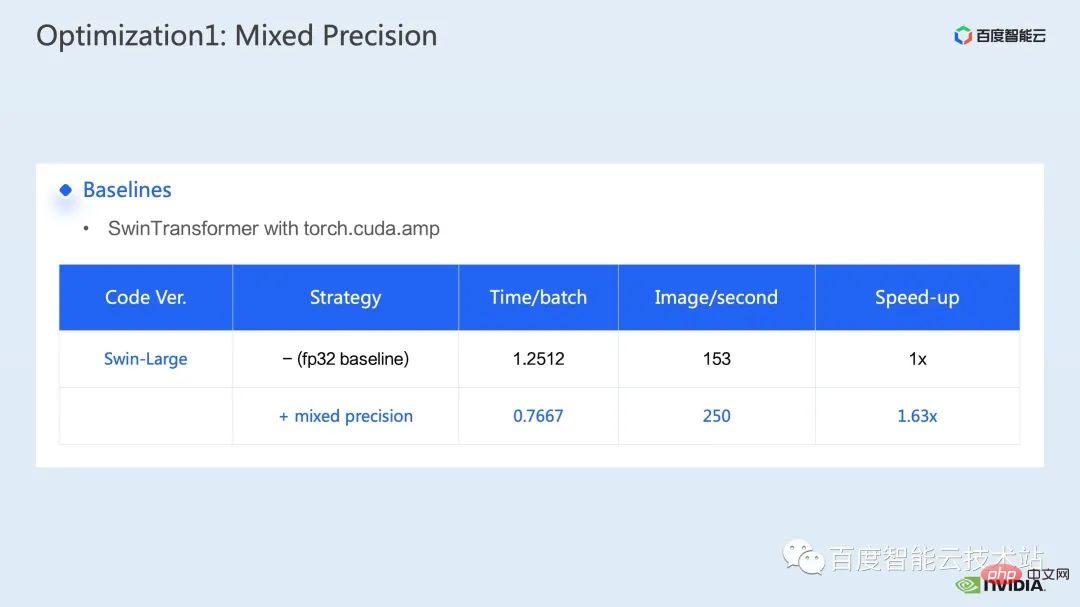
Here, we adopt a mixed precision solution. By using the mixed-precision mode of torch.cuda.amp, we can achieve a 1.63x throughput improvement.

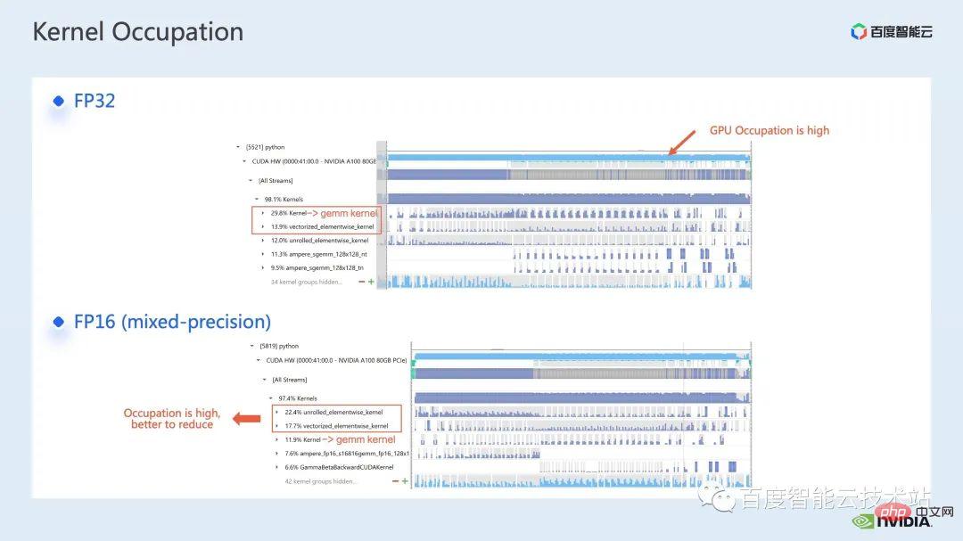
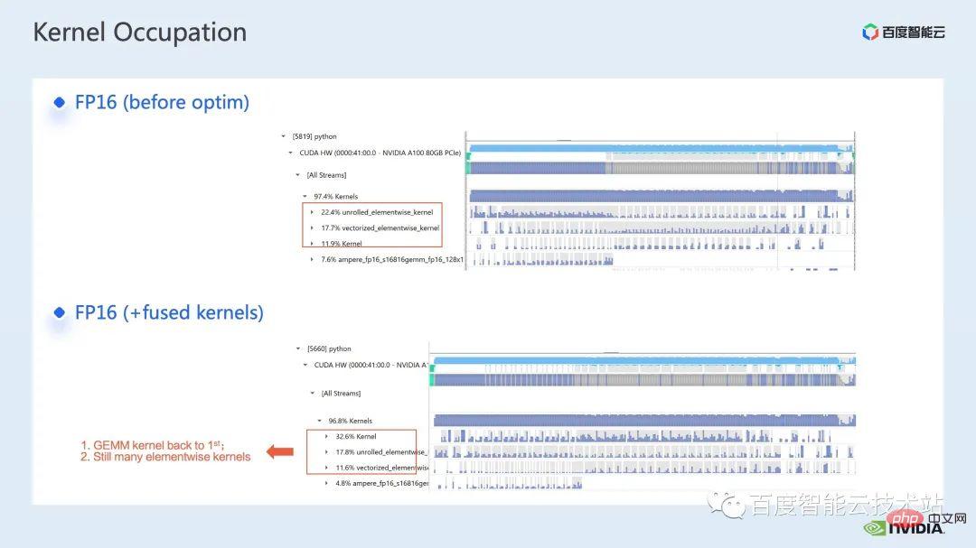
It can also be clearly seen in the profiling results that the matrix multiplication, which originally accounted for the highest number, has been optimized , the proportion in the entire timeline dropped to 11.9%. So far, the kernels with a relatively high proportion are elementwise kernels.

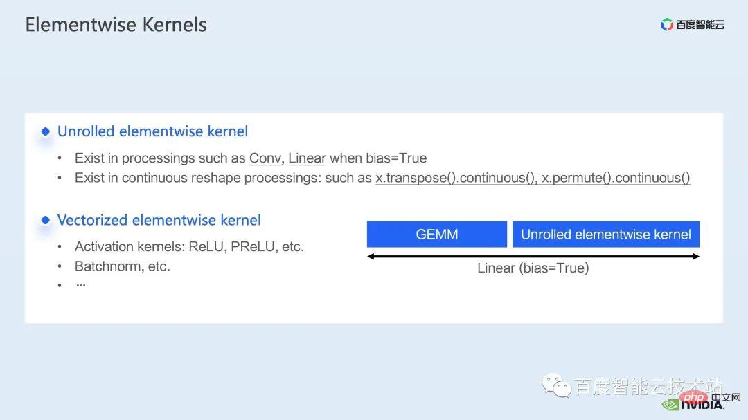
For the elementwise kernel, we first need to understand where the elementwise kernel will be used.

In the Elementwise kernel, the more common unrolled elementwise kernel and vectorized elementwise kernel. Among them, unrolled elementwise kernel is widely found in some biased convolutions or linear layers, as well as in some ops that ensure data continuity in memory.

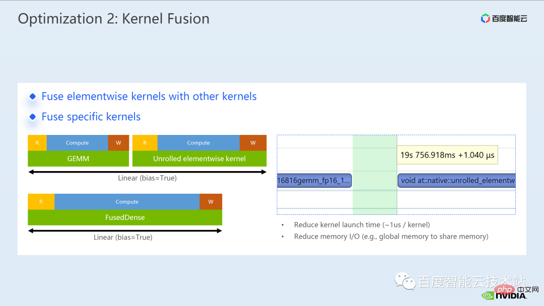
vectorized elementwise kernel often appears in the calculation of some activation functions, such as ReLU. If you want to reduce the large number of elementwise kernels here, a common approach is to perform operator fusion. For example, in matrix multiplication, we can reduce this part of the time overhead by fusing the elementwise operation with the operator of matrix multiplication.

Generally speaking, operator fusion can bring us two benefits:

One is to reduce the cost of kernel launch. As shown in the figure below, the execution of two cuda kernels requires two launches. This may cause a gap between the kernels and make the GPU idle. So if we merge two cuda kernels into one cuda kernel, on the one hand, we save a launch, and at the same time, we can avoid the generation of gaps.

Another benefit is that it reduces global memory access, because global memory access is very time-consuming, and results must be transferred between two independent cuda kernels through global memory. , fusing two cuda kernels into one kernel, we can transfer the results in registers or shared memory, thus avoiding one global memory write and read and improving performance.

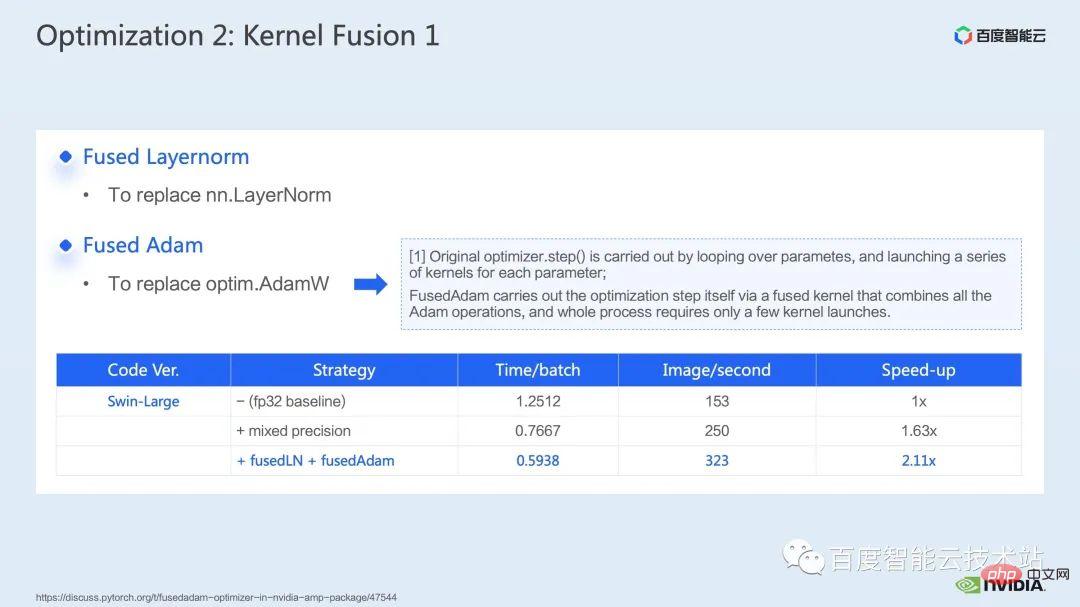
For operator fusion, our first step is to use the ready-made apex library to perform operations in Layernorm and Adam For fusion, we can see that through simple instruction replacement, we can enable apex's fused layernorm and fused Adam, thereby increasing the acceleration from 1.63 times to 2.11 times.

We can also see from the profling log that after operator fusion, the elementwise kernel accounts for the proportion of this timeline. The ratio has been greatly reduced, and matrix multiplication has once again become the kernel that accounts for the largest time.

In addition to using the existing apex library, we also developed manual fusion operators.

By observing the timeline and understanding the model, we found that there are unique window-related operations in Swin Transformer, such as window partition/shift/merge, etc., here A window shift requires calling two kernels, and the elementwise kernel is called after the shift is completed. Moreover, if such an operation needs to be performed before the attention module, there will be a corresponding reverse operation afterwards. Here, the roll_cuda_kernel called by window shift alone accounts for 4.6% of the entire timeline.

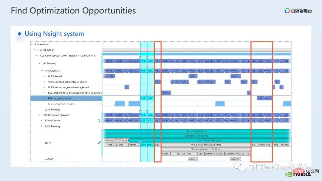
The operations just mentioned are actually just dividing the data, that is, the corresponding data will be divided into In a window, the corresponding original code is shown in the figure below.

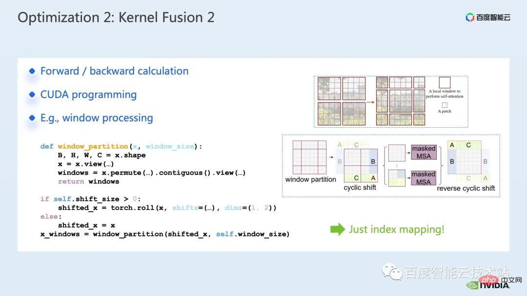
We found that this part of the operation is actually just index mapping. Therefore, we integrated this part Operator development. During the development process, we need to master the relevant knowledge of CUDA programming and write relevant codes for forward calculation and reverse calculation of operators.

How to introduce custom operators into pytorch, the official tutorial is given, we can follow the tutorial to write CUDA code, and after compilation, it can be used as a module Introduce the original model. It can be seen that by introducing our customized fusion operator, we can further increase the speedup to 2.19 times.

What follows is our fusion work on the mha part.

The Mha part is a large module in the transformer model, so optimizing it can often bring about greater acceleration effects. As can be seen from the figure, before operator fusion is performed, the proportion of operations in the mha part is 37.69%, which includes many elementwise kernels. If we can fuse related operations into a separate kernel with faster speed, the speedup can be further improved.

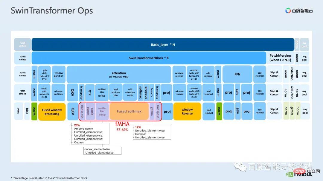
For Swin Transformer, in addition to query, key and value, mask and bias are passed in in the form of tensor. We have developed a module like fMHA, which can convert the original Several kernels are integrated. Judging from the calculations involved in the fMHA module, this module has significantly improved some shapes encountered in Swin Transformer.

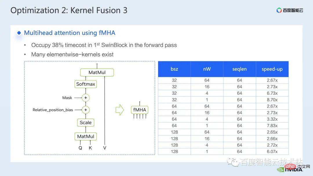
After using the fMHA module in the model, we can further increase the acceleration ratio by 2.85 times. The above is the training acceleration effect we achieved on a single card. Let's take a look at the training situation on a single machine with 8 cards. We can see that through the above optimization, we can increase the training throughput from 1612 to 3733, achieving an acceleration of 2.32 times.

For training optimization, we hope that the higher the acceleration ratio, the better. Correspondingly, we also hope that after the acceleration The performance can remain the same as before acceleration.

After superimposing the above several acceleration solutions, it can be seen that the convergence of the model is consistent with the original baseline. The convergence and accuracy of the model before and after optimization are improved. Consistency, proven on Swin-Tiny, Swin-Base and Swin-Large.

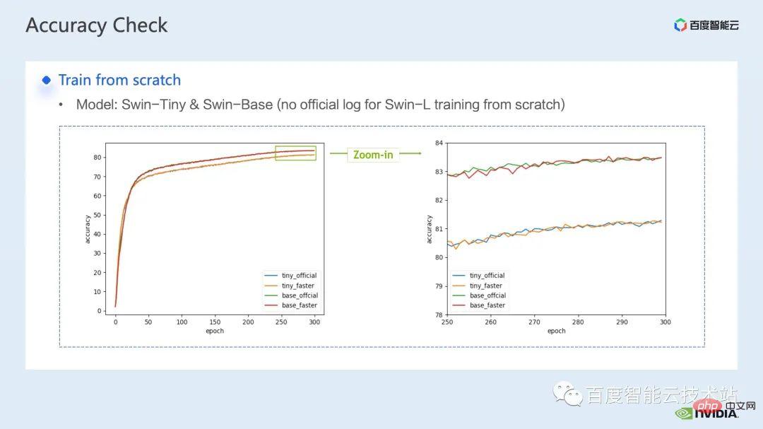
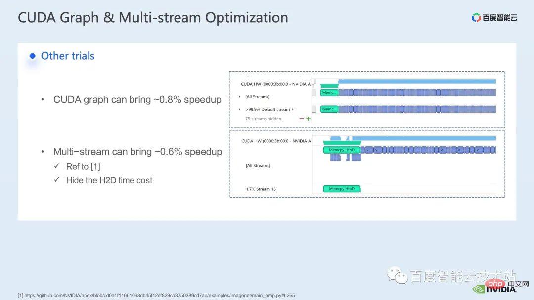
Regarding the training part, some other acceleration strategies including CUDA graph, multi-stream, etc. can all be used for Swin Transformer The performance has been further improved; in other aspects, we are currently introducing a mixed-precision solution, which is the strategy adopted by the Swin Transformer official repo; using a pure fp16 solution (ie, apex O2 mode) can achieve faster acceleration.

Although Swin does not have high communication requirements, for the training of multi-node large models, compared with the original distributed training, reasonable strategies are used to By hiding the communication overhead, further benefits can be obtained in multi-card training.

Next, I would like to ask my colleagues to introduce our acceleration solutions and effects in inference.

3. Swin Transformer Inference Optimization

Hello everyone , I am Chen Yu from NVIDIA's GPU computing expert team. Thank you very much for Tao Li's introduction on training acceleration. Next, let me introduce the acceleration on inference.

#Like training, the acceleration of inference is inseparable from the operator fusion solution. However, compared to training, operator fusion has better flexibility in reasoning, which is mainly reflected in two points:

• In reasoning The operator fusion does not need to consider the reverse direction, so the kernel development process does not need to consider saving the intermediate results required to calculate the gradient;
• The inference process allows preprocessing , we can calculate some operations that only require one calculation and can be used repeatedly, calculate them in advance, retain the results, and call them directly during each inference to avoid repeated calculations.

On the inference side, we can perform many operator fusions. Here are some common operators we use in the Transformer model. Integrated patterns and the tools needed to implement related patterns.

First of all, we list matrix multiplication and convolution separately because there is a large class of operator fusion around them. For fusion related to matrix multiplication, we can consider using cublas, cutlass, cudnn These three libraries; for convolution, we can use cudnn or cutlass. So for operator fusion of matrix multiplication, in the Transformer model, we summarize it as gemm elementwise operations, such as gemm bias, gemm bias activation function, etc. For this type of operator fusion, we can consider directly calling cublas or cutlass to fulfill.

In addition, if the op operations after our gemm are more complex, such as layernorm, transpose, etc., we can consider separating gemm and bias, and then integrating bias into In the next op, this makes it easier to call cublas to implement simple matrix multiplication. Of course, the pattern of integrating this bias with the next op generally requires us to write the cuda kernel by hand.

#Finally, there are some specific ops that also require us to fuse them by handwriting cuda kernel, such as layernorm shift window partition.

Since operator fusion requires us to design the cuda kernel more skillfully, we generally recommend analyzing the overall pipeline through the nsight system performance analysis tool first, giving priority to The hotspot module performs operator fusion optimization to achieve a balance between performance and workload.

So among the many operator fusion optimizations, we selected two operators with obvious acceleration effects. introduce.

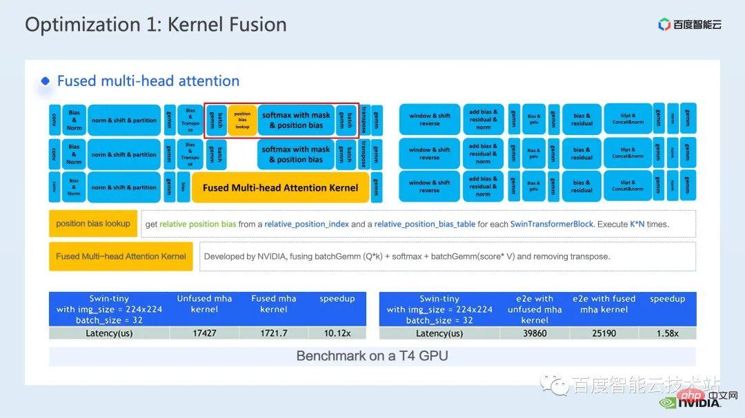
The first is the operator fusion of the mha part. We advance the position bias lookup operation to the preprocessing part to avoid performing a lookup every time inference. .

Then we merge batch gemm, softmax, and batch gemm into an independent fMHA kernel. At the same time, we integrate transpose related operations into fMHA kernel I/O operations. , a certain pattern of data reading and writing is used to avoid explicit transpose operations.

#It can be seen that after the fusion, this part has achieved a 10 times acceleration, and the end-to-end acceleration has also been achieved by 1.58 times.

Another operator fusion I want to introduce is the fusion of QKV gemm bias.

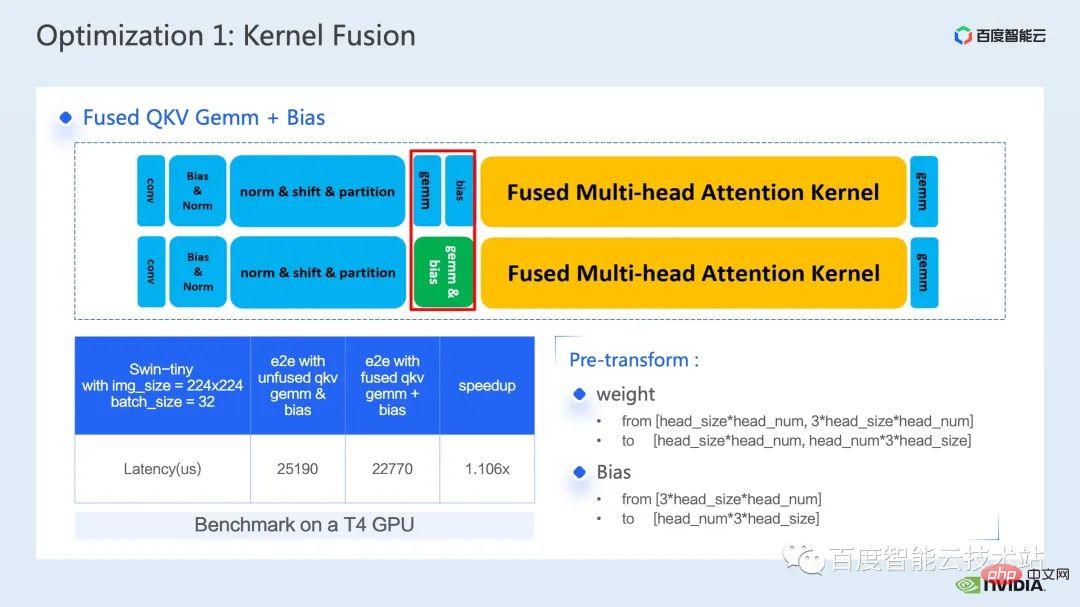
The fusion of gemm and bias is a very common fusion method. In order to cooperate with the fMHA kernel we mentioned earlier, we need to adjust weight and bias in advance. Make format changes.

The reason why I choose to introduce this operator fusion here is precisely because this advance transformation embodies what we mentioned earlier, inferential calculation. Due to the flexibility of sub-fusion, we can make some changes to the model's inference process that do not affect its accuracy, thereby achieving better operator fusion patterns and achieving better acceleration effects.

Finally, through the integration of QKV gemm bias, we can further achieve an end-to-end acceleration of 1.1 times.

The next optimization method is matrix multiplication padding.

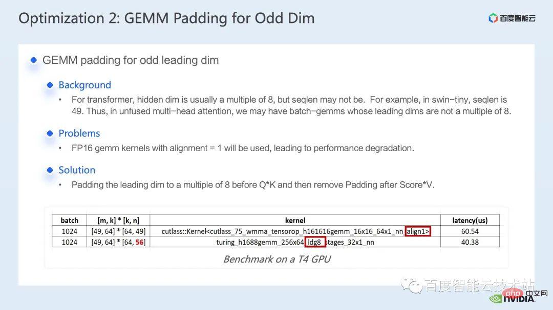
In the calculation of Swin Transformer, sometimes we encounter matrix multiplication with an odd main dimension. At this time, it is not conducive for our matrix multiplication kernel to perform vectorized reading and writing, thus making the kernel The operating efficiency becomes low. At this time, we can consider padding the main dimensions of the matrix participating in the operation to make it a multiple of 8. In this way, the matrix multiplication kernel can read and write 8 elements at a time with alignment=8. Method to perform vectorized reading and writing to improve performance.

As shown in the table below, after we padding n from 49 to 56, the latency of matrix multiplication dropped from 60.54us to 40.38us, achieving 1.5 times Speedup ratio.

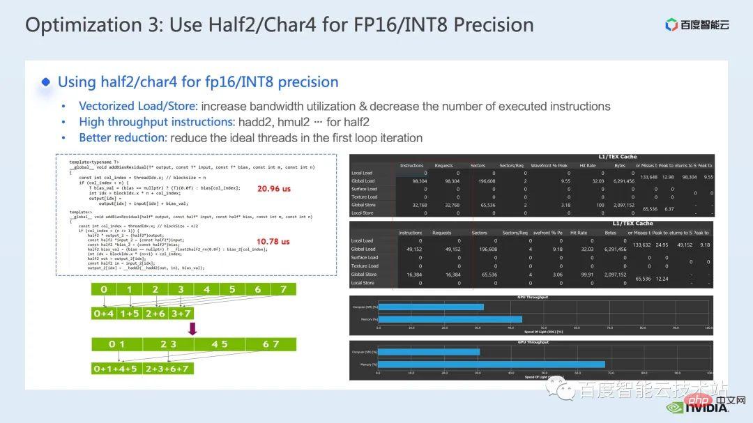
The next optimization method is to use data types such as half2 or char4.

The following code is an example of half2 optimization. It implements a simple operator fusion operation of adding bias and residual. You can see By using the half2 data type, compared to the half data class, we can reduce the latency from 20.96us to 10.78us, an acceleration of 1.94 times.

#So what are the general benefits of using the half2 data type? There are three main points:

The first benefit is that vectorized reading and writing can improve memory bandwidth utilization efficiency and reduce the number of memory access instructions; as shown on the right side of the figure below It shows that through the use of half2, the memory access instructions are reduced by half, and the SOL of memory is also significantly improved;

The second benefit is the combination of half2's proprietary High-throughput math instructions can reduce kernel latency. Both of these points have been reflected in this sample program;

#The third benefit is that when developing reduction-related kernels, using the half2 data type means One CUDA thread processes two elements at the same time, which can effectively reduce the number of idle threads and reduce the latency of thread synchronization.

The next optimization method is to use the register array cleverly.

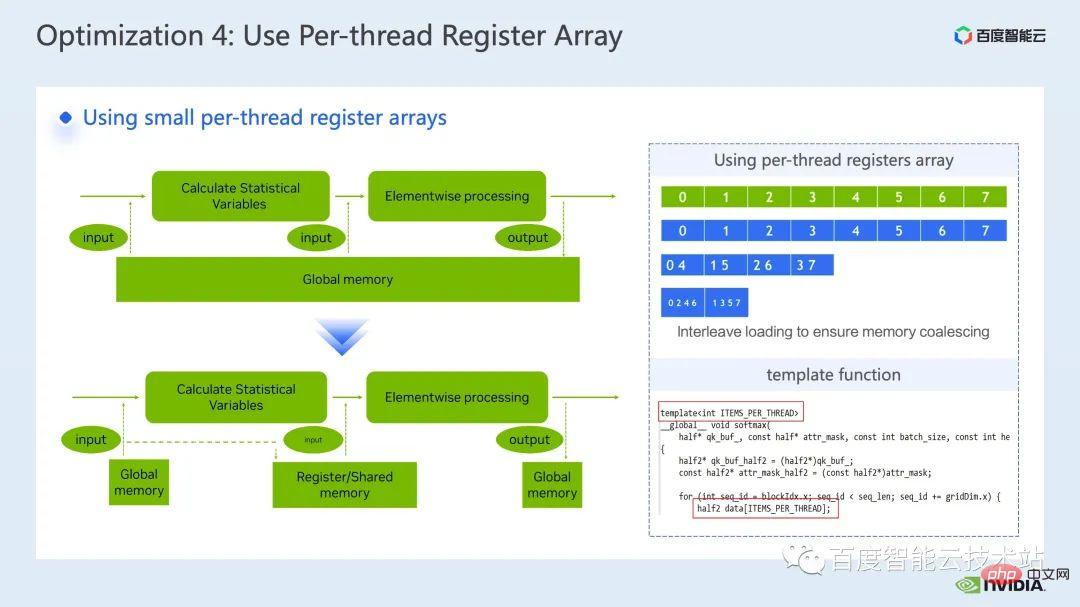
When we optimize common operators of Transformer models such as layernorm or softmax, we often need to use the same input data multiple times in a kernel, then Instead of reading from global memory every time, we can use a register array to cache data to avoid repeated reading of global memory.

Since the register is exclusive to each cuda thread, when designing the kernel, we need to set the elements that each cuda thread needs to cache in advance. number, thereby opening up a register array of corresponding size, and when allocating the elements responsible for each cuda thread, we need to ensure that we can achieve combined access, as shown on the upper right side of the figure below, when we have 8 threads, thread No. 0 It can process element No. 0. When we have 4 threads, thread No. 0 processes elements No. 0 and No. 4, and so on.

#We generally recommend using template functions to control the register array size of each cuda thread through template parameters.

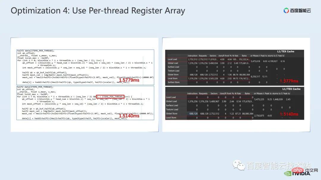
In addition, when using the register array, we need to ensure that our subscript is a constant. If it is a loop Variables are used as subscripts. We should try our best to ensure that loop expansion can be performed. This can prevent the compiler from placing data in local memory with high latency. As shown in the figure below, we add restrictions to the loop conditions, which can be seen through ncu report. , avoiding the use of local memory.

The last optimization method I want to introduce is INT8 quantization.

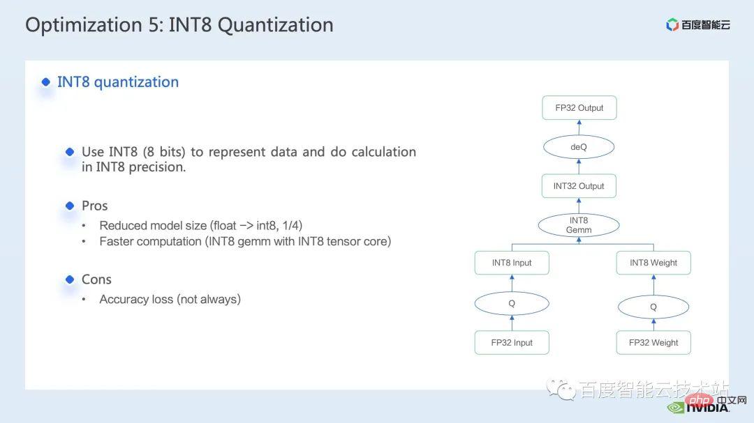
INT8 quantization is a very important acceleration method for inference acceleration. For Transformer based models, INT8 quantization can reduce memory consumption and bring better results. performance.

For Swin, by combining a suitable PTQ or QAT quantization scheme, you can achieve good acceleration while ensuring quantization accuracy. Generally, we perform int8 quantization, mainly to quantize matrix multiplication or convolution. For example, in int8 matrix multiplication, we will first quantize the original FP32 or FP16 input and weight into INT8 and then perform INT8 matrix multiplication and accumulate to INT32 data. Type-wise, this is where we would perform an inverse quantization operation and get the result of FP32 or FP16.

The more common tool for calling INT8 matrix multiplication is cublasLt. In order to achieve better performance, we need to go deeper. Let’s take a closer look at some features of the cublasLt api.

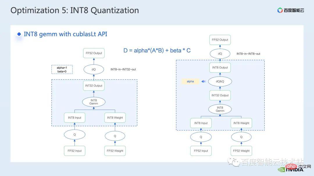
cublasLt For int8 matrix multiplication, two output types are provided, which are as shown on the left side of the figure below, output as INT32, or as shown on the right side of the figure below. Display, output in INT8, the calculation operation of cublasLt shown in the blue box in the figure.

It can be seen that compared to INT32 output, INT8 output will have an additional pair of inverse quantization and quantization operations, which will generally bring more There is a loss of accuracy, but because INT8 output has 3/4 less data volume than INT32 output when writing to global memory, the performance will be better, so there is a tradeoff between accuracy and performance.

So for Swin Transformer, we found that with QAT, INT8 output will ensure accuracy under the premise of achieving a good acceleration ratio, because we use INT8 output scheme.

##In addition, regarding the INT8 matrix multiplication in cublasLt, you also need to consider the layout of the data. cublasLt supports two There is one layout, an IMMA-specific layout, which involves some more complex formats, and only supports NT-gemm in this layout. The other is a regular column-first layout, which supports TN-gemm in this layout. .

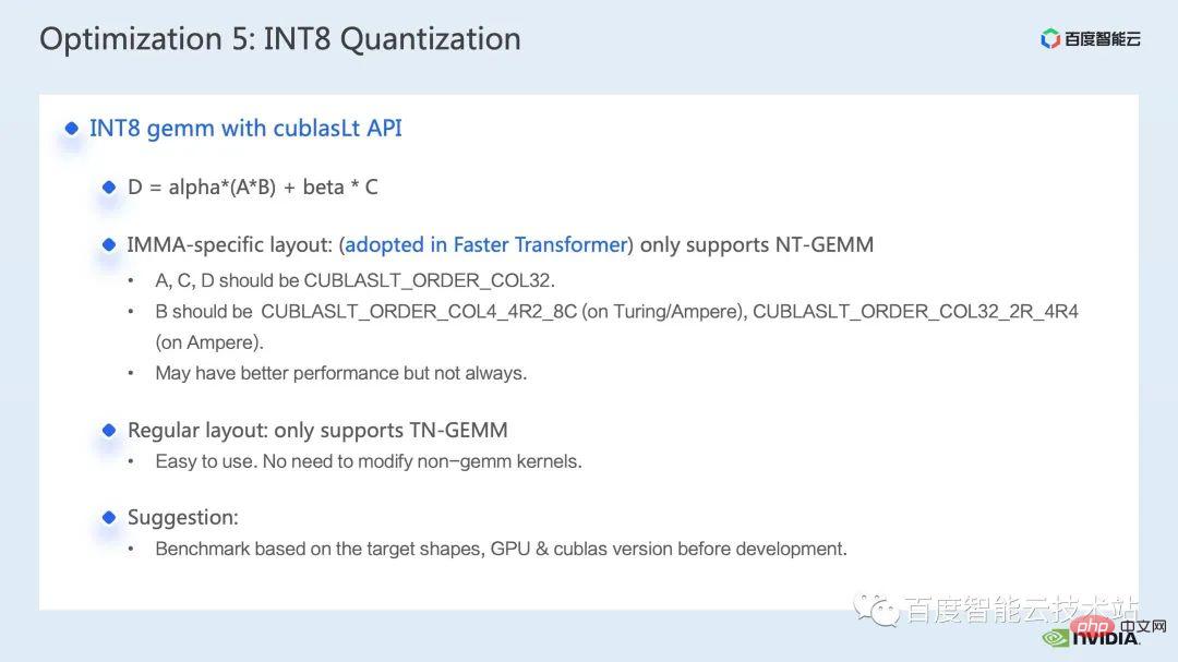
Generally speaking, using column-first layout will be more conducive to the development of the entire pipeline code, because if we use IMMA-specific layout, we may need to be compatible with this layout Many additional operations, as well as upstream and downstream kernels, also need to be compatible with this special layout. However, IMMA-specific layout may have better performance on matrix multiplication of some sizes, so if we want to try to build int8 reasoning, it is recommended that we do some benchmarks first to better understand the performance and development ease. Make trade-offs.

#In FasterTransformer we use IMMA-specific layout. So next, we take the IMMA-specific layout as an example to briefly introduce the basic construction process of cublasLt int8 matrix multiplication, as well as some development techniques.

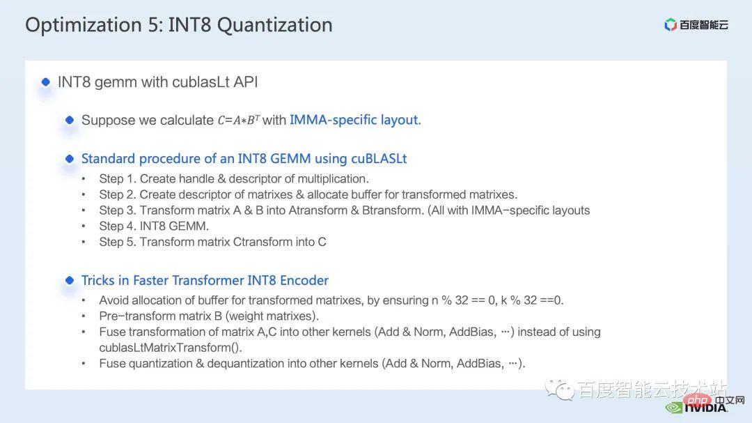
##cublasLt int8 The basic construction process of matrix multiplication can be divided into 5 steps:

• First we need to create handles and multiplication descriptors;
• Next we create a matrix for each matrix Descriptor;
• Because generally our input is a regular layout, so we need to perform layout conversion on the regular layout matrix to make it IMMA- specific layout;
• Then perform int8 matrix multiplication. After getting the result, we can consider continuing to use this result for downstream multiplication calculations, so as to avoid transformation There will be the overhead of regular layout;
• Only the result of the last matrix multiplication, we need to convert the regular layout for output.

The above describes the construction process under the IMMA-specific layout. You can see that there are many restrictions. In order to avoid the impact of these limitations on performance, we adopt the following techniques in Faster Transformer:

• First of all, the IMMA-specific layout is specific to the matrix size requirements, in order to avoid the need to allocate additional space during the inference process, we will allocate a buffer that conforms to the IMMA-specific layout size in advance;
• Then, Since weight can be processed and reused once, we will perform layout transformation on weight (equivalent to the B matrix in multiplication) in advance to avoid repeatedly changing weight during the inference process;
• The third trick is that for A and C that have to undergo special layout transformation, we will merge the transformation with the upstream or downstream op to hide this part of the overhead;
• The last point has nothing to do with the layout, but the quantization and inverse quantization operations that are necessary for int8 matrix multiplication. We will also use operator fusion to hide its latency. .

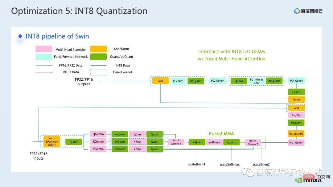
The following is a schematic diagram of the INT8 process we use in Faster Transformer. You can see that all Matrix multiplication has become an int8 data type. Corresponding quantization and inverse quantization nodes will be inserted before and after each int8 matrix multiplication. Then for operations such as adding bias, adding residuals or layernorm, we still retain the original FP32 or FP16 data type. Of course Its I/O may be int8, which will provide better I/O performance than FP16 or FP32.

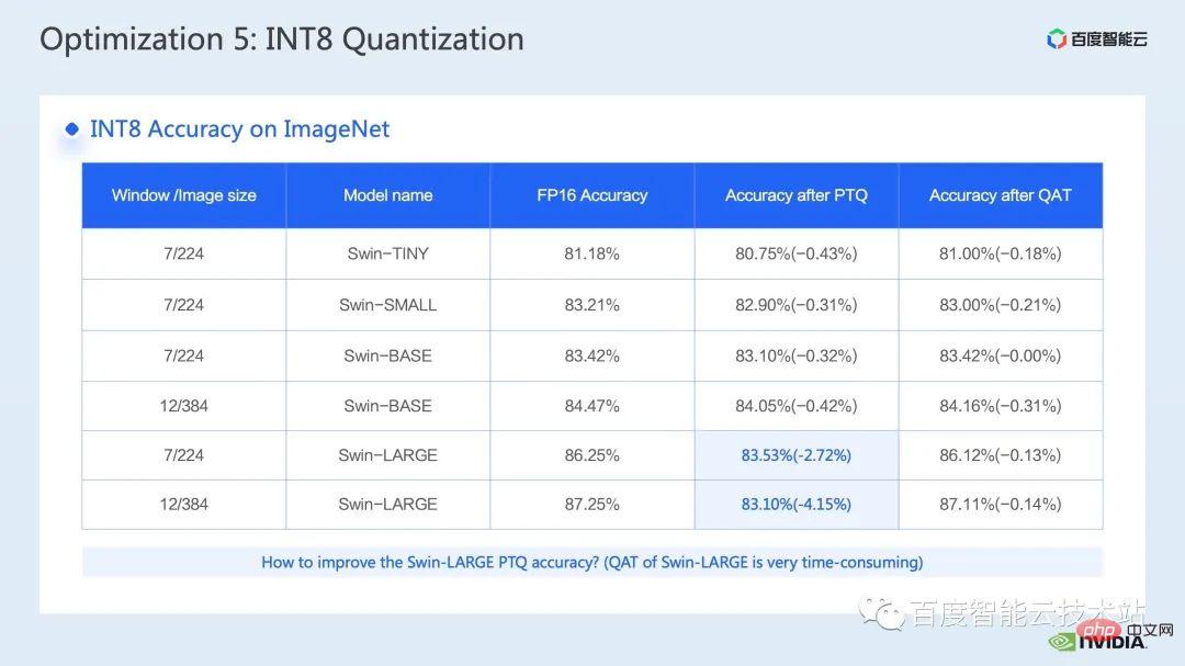
What is shown here is the accuracy of Swin Transformer int8 quantization. Through QAT we can ensure that the accuracy loss is within one thousandth Within 5.

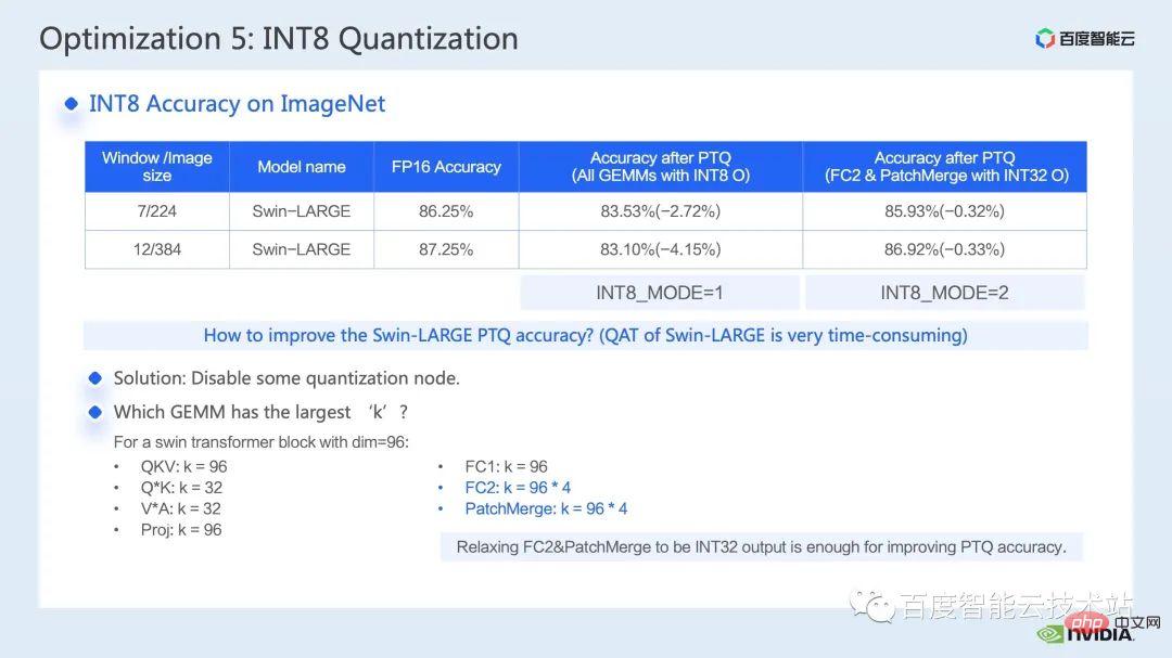
In the PTQ column, we can see that the point drop of Swin-Large is more serious. Generally, we can consider using it if it corresponds to serious point drop problems. Reduce some quantization nodes to improve quantization accuracy. Of course, this may weaken the acceleration effect.

In FT, we can disable inverse quantization before output of int8 matrix multiplication in FC2 and PatchMerge and quantization nodes (that is, using int32 output) to further improve the quantization accuracy. It can be seen that under this optimization operation, the PTQ accuracy of swin-large has also been significantly improved.

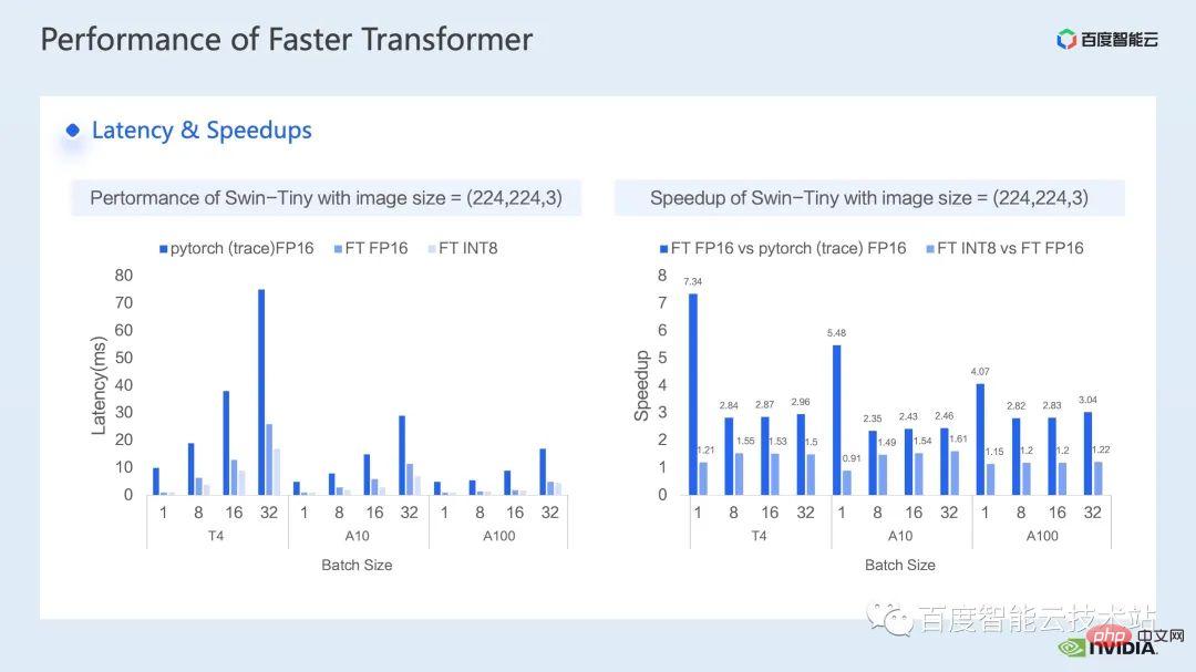
The following is the acceleration effect we achieved on the inference side. We tested different models of GPU T4, A10, and A100. The performance comparison with the pytorch FP16 implementation was performed above.

The left side of the figure below is the latency comparison between optimization and pytorch, and the right figure is the acceleration ratio between FP16 and pytorch after optimization, and the acceleration ratio between INT8 optimization and FP16 optimization. It can be seen that through optimization, we can achieve an acceleration of 2.82x ~ 7.34x relative to pytorch in terms of FP16 accuracy. Combined with INT8 quantization, we can further achieve an acceleration of 1.2x ~ 1.5x on this basis.

4. Swin Transformer Optimization Summary

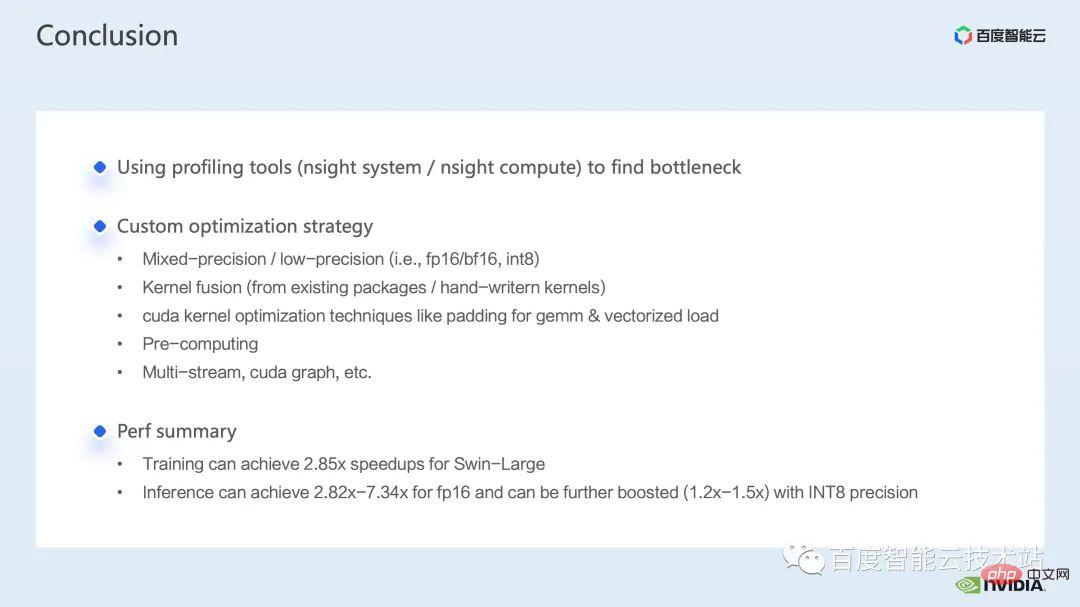
Finally, let’s summarize. In this sharing, we introduced how to find performance bottlenecks through the nsight system performance analysis tool, and then introduced a series of training inference acceleration techniques for performance bottlenecks, including 1. Hybrid Precision training/low-precision reasoning, 2. Operator fusion, 3. cuda kernel optimization techniques: such as matrix zero padding, vectorized reading and writing, clever use of register arrays, etc. 4. Some preprocessing is used in inference optimization to improve our Computational process; we also introduced some applications of multi-stream and cuda graph.

Combined with the above optimization, we used the Swin-Large model as an example to achieve an acceleration ratio of 2.85x for a single card and 2.32x for an 8-card model. ratio; in terms of reasoning, taking the Swin-tiny model as an example, it achieved an acceleration ratio of 2.82x ~ 7.34x under FP16 accuracy. Combined with INT8 quantization, it further achieved an acceleration ratio of 1.2x ~ 1.5x.

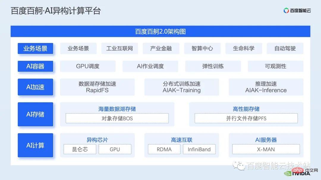
The above acceleration methods for large visual model training and inference have been implemented in AIAK of Baidu Baige AI heterogeneous computing platform Implemented in the acceleration function, everyone is welcome to use it.

The above is the detailed content of How to use large visual models to accelerate training and inference?. For more information, please follow other related articles on the PHP Chinese website!