


Classifying time series is one of the common tasks for applying machine and deep learning models. This article will cover 8 types of time series classification methods. This ranges from simple distance or margin based methods to methods using deep neural networks. This article is intended to serve as a reference article for all time series classification algorithms.
Before covering various types of time series (TS) classification methods, we first unify the concept of time series. TS can be divided into Be univariate or multivariate TS.
The data set of single or multiple TS usually contains an ordered set of single or multiple TS. Furthermore, datasets usually contain a label vector represented by a single encoding, the length of which represents the labels of different classes.
The goal of TS classification is defined by training any classification model on a given dataset so that the model can learn the probability distribution of the provided dataset. That is, the model should learn to correctly assign class labels when given a TS.
Distance-based or nearest-neighbor-based TS classification methods use various distance-based metrics to classify the given data. It is a supervised learning technique in which the prediction result of a new TS depends on the label information of the known time series to which it is most similar.
A distance metric is a function that describes the distance between two or more time series and is decisive. Typical distance measures are:
After deciding on the metric, the k-nearest neighbor (KNN) algorithm is usually applied, which measures the distance between the new TS and all TS in the training data set. After calculating all distances, select the k closest ones. Finally the new TS is assigned to the class to which the majority of the k nearest neighbors belong.
While the most popular norms are definitely the p-norm, especially the Euclidean distance, they have two main disadvantages that make them less suitable for TS classification tasks. Since the norm is only defined for two TSs of the same length, it is not always possible to obtain sequences of equal length in practice. The norm only compares two TS values at each time point independently, but most TS values are correlated with each other.
And DTW can solve the two limitations of p norm. Classic DTW minimizes the distance between two time series points whose timestamps may be different. This means that slightly shifted or distorted TSs are still considered similar. The figure below visualizes the difference between p-norm based metrics and how DTW works.
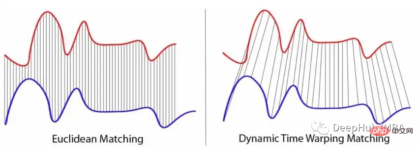
Combined with KNN, DTW is used as the baseline algorithm for various benchmark evaluations of TS classification.
KNN can also be implemented using a decision tree method. For example, the neighbor forest algorithm models a forest of decision trees that uses distance measures to partition TS data.
Interval-based methods usually divide the TS into multiple different intervals. Each subsequence is then used to train a separate machine learning (ML) classifier. A set of classifiers will be generated, each classifier acting on its own interval. Computing the most common class among separately classified subseries returns the final label for the entire time series.
The most famous representative of the interval-based model is the Time Series Forest. A TSF is a collection of decision trees built on random subsequences of the initial TS. Each tree is responsible for assigning a class to a range.
This is done by calculating summary features (usually the mean, standard deviation, and slope) to create a feature vector for each interval. Decision trees are then trained based on the computed features and predictions are obtained by majority voting of all trees. The voting process is necessary because each tree only evaluates a certain subsequence of the initial TS.
In addition to TSF, there are other interval-based models. Variants of TSF use additional features such as median, interquartile range, minimum and maximum values of the subseries. Compared with the classic TSF algorithm, there is a rather complex algorithm called the Random Interval Spectral Ensemble (RISE) algorithm.
The RISE algorithm differs from the classic TS forest in two aspects.
In RISE technology, each decision tree is built on a different set of Fourier, autocorrelation, autoregressive and partial autocorrelation features. The algorithm works as follows:
Select the first random intervals of TS and calculate the above features on these intervals. A new training set is then created by combining the extracted features. Based on these, a decision tree classifier is trained. These steps are finally repeated using different configurations to create an ensemble model, which is a random forest of a single decision tree classifier.
Dictionary-based algorithm is another type of TS classifier, which is based on the structure of the dictionary. They cover a large number of different classifiers and can sometimes be used in combination with the above classifiers.
Here is a list of dictionary-based methods covered:
This type of method usually first converts TS into a symbol sequence and extracts "WORDS" from it through a sliding window. The final classification is then done by determining the distribution of "WORDS", which is usually done by counting and sorting the "WORDS". The theory behind this approach is that time series are similar, meaning they belong to the same class if they contain similar "WORDS". The main process of dictionary-based classifiers is usually the same.
Here is a list of the most popular dictionary-based classifiers:
The Bag-of-Patterns (BOP) algorithm works similarly to the Bag-of-Words algorithm used for text data classification. This algorithm counts the number of times a word occurs.
The most common technique for creating words from numbers (here raw TS) is called Symbolic Aggregation Approximation (SAX). The TS is first divided into different blocks, each block is then normalized, meaning it has a mean of 0 and a standard deviation of 1.
Usually the length of a word is longer than the number of real values in the subsequence. Therefore, binning is further applied to each block. The average actual value for each bin is then calculated and mapped to a letter. For example, all values below -1 are assigned the letter "a", all values above -1 and below 1 are "b", and all values above 1 are "c". The image below visualizes this process.
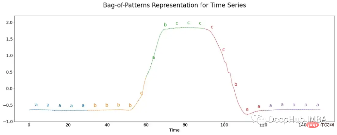
Here each segment contains 30 values, these values are divided into groups of 6, each group is assigned three possible letters, forming a five-letter word. The number of occurrences of each word is finally summarized and used for classification by inserting them into the nearest neighbor algorithm.
Contrary to the idea of the above BOP algorithm, in the BOP algorithm, the original TS is discretized into letters and then words, and similar Fourier coefficients can be applied to the TS method.
The most famous algorithm is Symbolic Fourier Approximation (SFA), which can be divided into two parts.
Compute the discrete Fourier transform of TS while retaining a subset of the calculated coefficients.
Each column of the resulting matrix is independently discretized, converting TS subsequences of TS into single words.
Based on the above preprocessing, various algorithms can be used to further process the information to obtain TS predictions.
The working principle of the Bag-of-SFA-Symbols (BOSS) algorithm is as follows:
Variants of the BOSS algorithm include many variations:
The BOSS Ensemble algorithm is often used to build multiple single BOSS models, each model in They vary in terms of parameters: word length, alphabet size, and window size. Capture patterns of various lengths with these configurations. A large number of models are obtained by grid-searching the parameters and retaining only the best classifiers.
The BOSS in Vector Space (BOSSVS) algorithm is a variation of the individual BOSS method using the vector space model, which computes a histogram for each class and computes Term frequency-inverse document frequency (TF-IDF) matrix. The classification is then obtained by finding the class with the highest cosine similarity between the TF-IDF vector of each class and the histogram of the TS itself.
The Contractable BOSS (cBOSS) algorithm is computationally much faster than the classic BOSS method.
Acceleration is achieved by not performing a grid search on the entire parameter space but on randomly selected samples from it. cBOSS uses a subsample of the data for each base classifier. cBOSS improves memory efficiency by considering only a fixed number of best base classifiers instead of all classifiers above a certain performance threshold.
The next variant of the BOSS algorithm is Randomized BOSS (RBOSS). This method adds a stochastic process in the selection of the sliding window length and cleverly aggregates the predictions of individual BOSS classifiers. This is similar to the cBOSS variant, reducing computation time while still maintaining baseline performance.
The TS Classifier Extraction (WEASEL) algorithm can improve the performance of the standard BOSS method by using sliding windows of different lengths in the SFA transformation. Similar to other BOSS variants, it uses window sizes of various lengths to convert TS into feature vectors, which are then evaluated by a KNN classifier.
WEASEL uses a specific feature derivation method, filtering out the most relevant features by using only non-overlapping subsequences of each sliding window applying the χ2 test.
Combine WEASEL with Multivariate Unsupervised Symbols (WEASEL MUSE) to extract and filter multivariate features from TS by encoding contextual information into each feature.
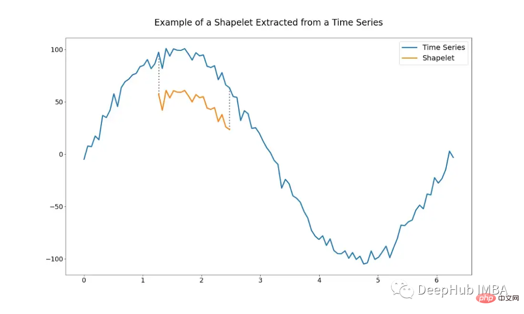
The shapelet-based method uses the idea of subsequences of the initial time series (ie shapelets). Shapelets are chosen in order to use them as representatives of classes, which means that shapelets contain the main characteristics of a class that can be used to distinguish different classes. In the optimal case, they can detect local similarities between TS within the same class.
The following figure shows an example of a shapelet. It's just a subsequence of the entire TS.
Using algorithms based on shapelets requires determining which shapelets to use. It is possible to select by hand making a set of shapelets, but this can be very difficult. Shapelets can also be selected automatically using various algorithms.
Shapelet Transform is an algorithm based on Shapelet extraction proposed by Lines et al. It is one of the most commonly used algorithms at present. Given a TS of n real-valued observations, a shapelet is defined by a subset of TS of length l.
The minimum distance between a shapelet and the entire TS can be measured using Euclidean distance - or any other distance metric - the distance between the shapelet itself and all shapelets of length l starting from the TS.
Then the algorithm selects the k best shapelets whose lengths fall within a certain range. This step can be viewed as some kind of univariate feature extraction, with each feature defined by the distance between the shapelet and all TS in the given dataset. The shapelets are then ranked based on some statistics. These are usually f-statistics or χ² statistics, which rank shapelets according to their ability to distinguish classes.
After completing the above steps, any type of ML algorithm can be applied to classify the new data set. For example, knn-based classifiers, support vector machines or random forests, etc.
Another problem with finding ideal shapelets is the terrible time complexity, which increases exponentially with the number of training samples.
Shapelet learning-based algorithm attempts to solve the limitations of algorithms based on Shapelet extraction. The idea is to learn a set of shapelets capable of distinguishing classes, rather than extracting them directly from a given dataset.
Doing this has two main advantages:
But this approach also has some drawbacks with using a differentiable minimization function and the selected classifier Shortcomings.
To replace the Euclidean distance, we must rely on differentiable functions, so that shapelets can be learned through gradient descent or backpropagation algorithms. The most common relies on the LogSumExp function, which smoothly approximates the maximum by taking the logarithm of the sum of the exponents of its arguments. Because the LogSumExp function is not strictly convex, the optimization algorithm may not converge correctly, which means it may lead to bad local minima.
And since the optimization process itself is the main component of the algorithm, multiple hyperparameters need to be added for tuning.
But this method is very useful in practice and can generate some new insights into the data.
A slight variation of the shapelet-based algorithm is the kernel-based algorithm. Learn and use random convolution kernels (the most common computer vision algorithm), which extract features from a given TS.
The Random Convolution Kernel Transform (ROCKET) algorithm is specially designed for this purpose. . It uses a large number of kernels that vary in length, weight, bias, dilation, and padding, and are randomly created from a fixed distribution.
After selecting the kernel, a classifier is also needed that can select the most relevant features to distinguish classes. Ridge regression (an L2 regularized variant of linear regression) was used in the original paper to perform predictions. There are two benefits to using it, firstly its computational efficiency, even for multi-class classification problems, and secondly the simplicity of fine-tuning unique regularization hyperparameters using cross-validation.
One of the core advantages of using kernel-based algorithms or ROCKET algorithms is that the computational cost of using them is quite low.
Feature-based methods can generally cover most algorithms that use some kind of feature extraction for a given time series, and then predictions are performed by a classification algorithm.
Regarding features, from simple statistical features to more complex Fourier-based features. A large number of such features can be found in hctsa (https://github.com/benfulcher/hctsa), but trying and comparing each feature can be an impossible task, especially for larger datasets. Therefore, the typical time series feature (catch22) algorithm was proposed.
This method aims to infer a small TS feature set, which not only requires strong classification performance, but also further minimizes redundancy. catch22 selected a total of 22 features from the hctsa library (the library provides more than 4000 features).
The developers of this method obtained a kid that still maintains excellent performance by training different models on 93 different datasets to obtain 22 features and evaluating the best-performing TS features on them set. The classifier on it can be freely chosen, which makes it another hyperparameter to tune.
Another feature-based method is the Matrix Profile (MP) classifier, which is an interpretable MP-based TS classifier that can maintain baseline performance. while providing interpretable results.
The designers extracted a model named Matrix Profile from the shapelet-based classifier. The model represents all distances between a subsequence of a TS and its nearest neighbors. In this way, MP can effectively extract the features of TS, such as motifs and discords. Motifs are subsequences of TS that are very similar to each other, while discords describe sequences that are different from each other.
As a theoretical classification model, any model can be used. The developers of this method chose decision tree classifiers.
In addition to the two mentioned methods, sktime also provides some more feature-based TS classifiers.
Model Ensemble is not a stand-alone algorithm per se, but a technique that combines various TS classifiers to create better combined predictions. Model ensembles reduce variance by combining multiple individual models, similar to a random forest using a large number of decision trees. And using various types of different learning algorithms leads to a broader and more diverse set of learned features, which in turn leads to better class discrimination.
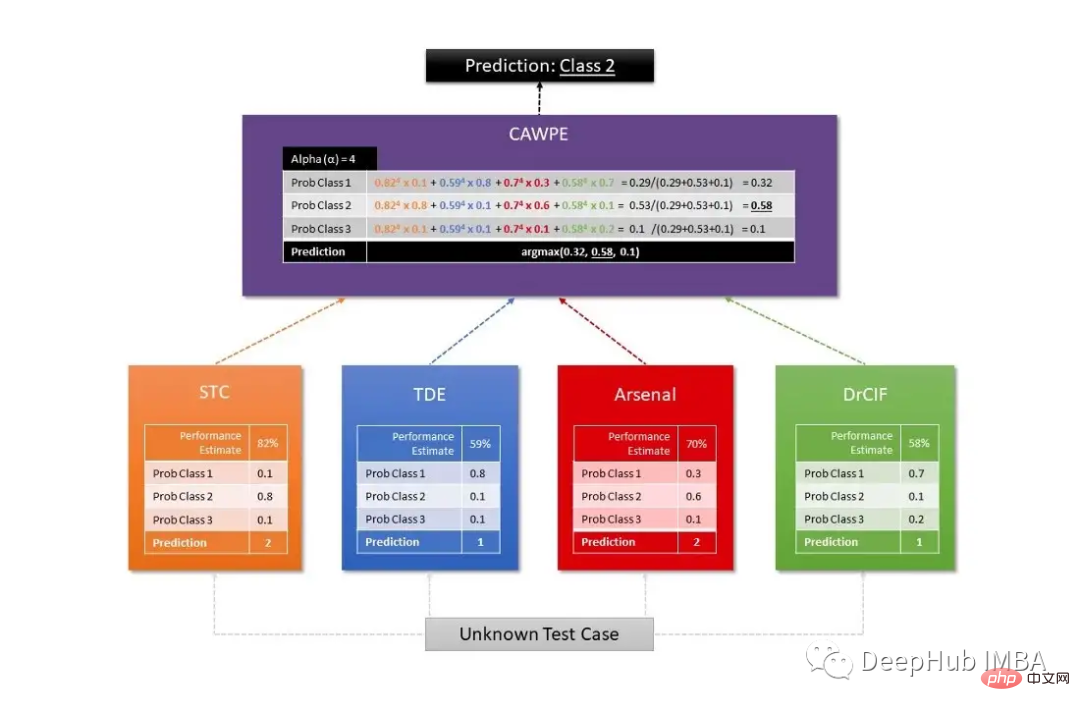
The most popular model ensemble is Hierarchical Vote Collective of Transformation-based Ensembles (HIVE-COTE). It exists in many different kinds of similar versions, but what they all have in common is the combination of information from different classifiers, i.e. predictions, by using a weighted average for each classifier.
Sktime uses two different HIVE-COTE algorithms, the first of which combines probabilities per estimator, including a shapelet transform classifier (STC), a TS forest, a RISE and a cBOSS . The second is defined by a combination of STC, Diverse Canonical Interval Forest Classifier (DrCIF, a variant of TS Forest), Arsenal (a collection of ROCKET models), and TDE (a variant of the BOSS algorithm).
The final prediction is obtained by the CAWPE algorithm, which assigns weights to each classifier obtained by the relative estimated quality of the classifiers found on the training data set.
The following figure is a common diagram used to visualize the working structure of the HIVE-COTE algorithm:
About Algorithms based on deep learning could write a long article of their own to explain all the details about each architecture. However, this article only provides some commonly used TS classification benchmark models and techniques.
While deep learning-based algorithms are very popular and widely studied in fields such as computer vision and NLP, they are less common in the field of TS classification. Fawaz et al. An exhaustive study of current existing methods in their paper on deep learning for TS classification: Summary More than 60 neural network (NN) models with six architectures were studied:
Most of the above models were originally developed for different use cases. So it needs to be tested according to different use cases.
Also launched in 2020 is the InceptionTime network. InceptionTime is an ensemble of five deep learning models, each of which was created by InceptionTime first proposed by Szegedy et al. These initial modules apply multiple filters of different lengths to the TS simultaneously, while extracting relevant features and information from shorter and longer subsequences of the TS. The following figure shows the InceptionTime module.
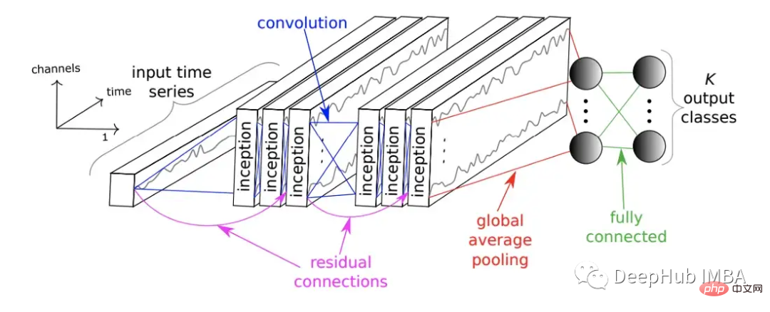
It consists of multiple initial modules stacked in a feed-forward manner and connected with the residuals. Finally, global average pooling and fully connected neural networks generate prediction results.
The figure below shows the working of a single initial module.
The large list of algorithms, models and techniques summarized in this article will not only help understand the vast field of time series classification methods, but I hope it will be useful to you. help
The above is the detailed content of Summary of eight time series classification methods. For more information, please follow other related articles on the PHP Chinese website!


![[Web front-end] Node.js quick start](https://img.php.cn/upload/course/000/000/067/662b5d34ba7c0227.png)


