

 Backend Development
Python Tutorial
Summary of common methods for Python time series data manipulation
Backend Development
Python Tutorial
Summary of common methods for Python time series data manipulation
Summary of common methods for Python time series data manipulation

Time series data is a type of data collected over a period of time. It is often used in fields such as finance, economics, and meteorology, and is often analyzed to understand trends and patterns over time.
Pandas is a powerful and popular data manipulation library in Python, especially suitable for processing time series data. It provides a set of tools and functions to easily load, manipulate and analyze time series data.
In this article, we introduce indexing and slicing of time series data, resampling and rolling window calculations, and other useful common operations, which are key techniques for manipulating time series data using Pandas.
Data types
Python
In Python, there is no built-in data type specifically for representing dates. Under normal circumstances, the datetime object provided by the datetime module is used for date and time operations.
import datetime

t = datetime.datetime.now()
print(f"type: {type(t)} and t: {t}")
#type: <class 'datetime.datetime'> and t: 2022-12-26 14:20:51.278230
Generally, we use strings to store dates and times. So we need to convert these strings into datetime objects when using them.
Generally, the time string has the following format:
- YYYY-MM-DD (e.g. 2022-01-01)
- YYYY/MM/DD (e.g. 2022/01/01)
- DD-MM-YYYY (e.g. 01-01-2022)
- DD/MM/YYYY (e.g. 01/01/2022)
- MM-DD-YYYY (e.g. 01-01-2022)
- MM/DD/YYYY (e.g. 01/01/2022)
- HH:MM:SS (e.g. 11:30 :00)
- HH:MM:SS AM/PM (e.g. 11:30:00 AM)
- HH:MM AM/PM (e.g. 11:30 AM)
The strptime function takes a string and a format string as parameters and returns a datetime object.
string = '2022-01-01 11:30:09'
t = datetime.datetime.strptime(string, "%Y-%m-%d %H:%M:%S")
print(f"type: {type(t)} and t: {t}")
#type: <class 'datetime.datetime'> and t: 2022-01-01 11:30:09
The format string is as follows:
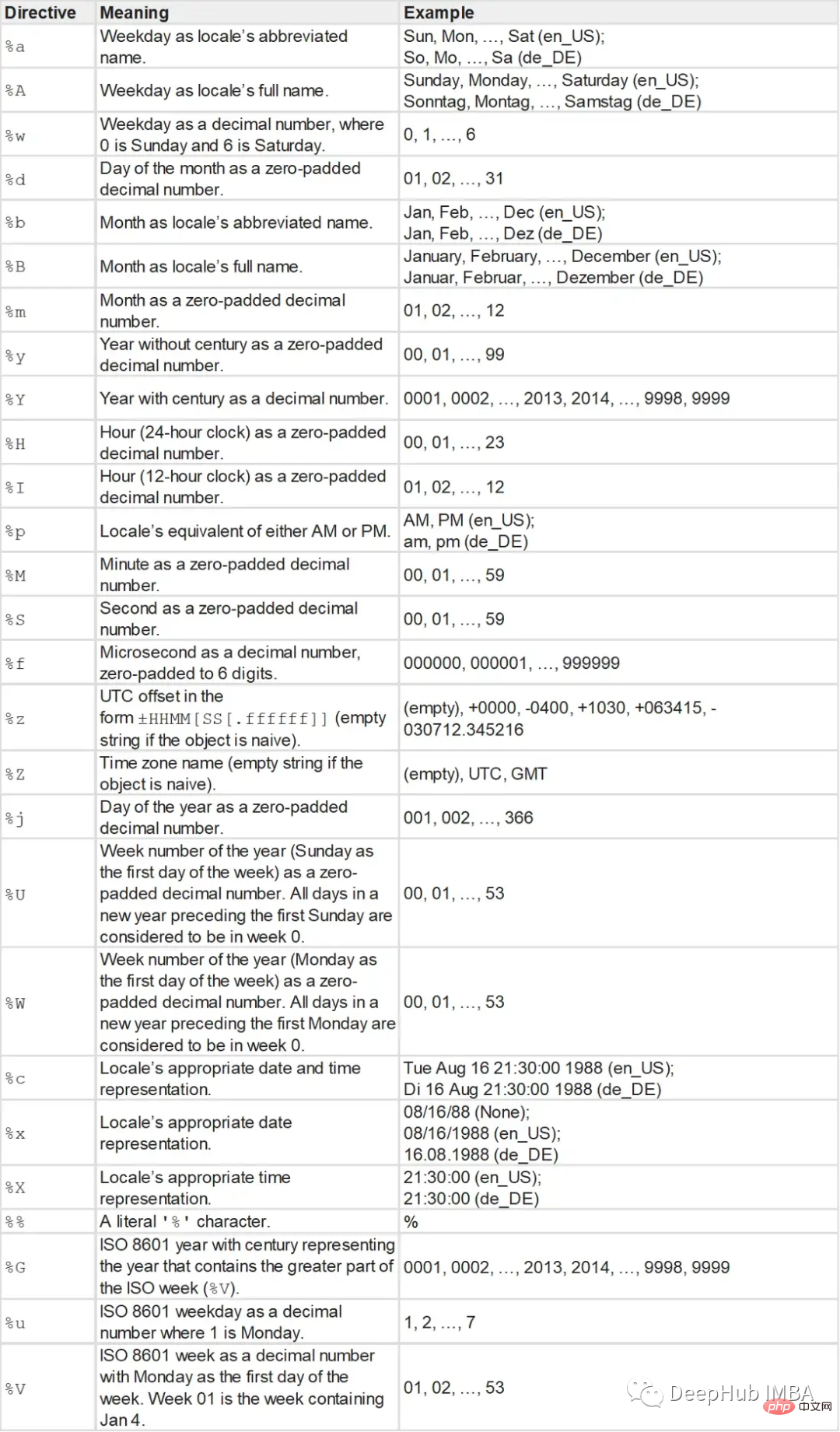
You can also use the strftime function to convert the datetime object back to a string representation in a specific format.
t = datetime.datetime.now()
t_string = t.strftime("%m/%d/%Y, %H:%M:%S")
#12/26/2022, 14:38:47

t_string = t.strftime("%b/%d/%Y, %H:%M:%S")
#Dec/26/2022, 14:39:32
Unix time (POSIX time or epoch time) is a system that represents time as a single numerical value. It represents the number of seconds elapsed since 00:00:00 Coordinated Universal Time (UTC) on Thursday, January 1, 1970.
Unix time and timestamp are often used interchangeably. Unix time is the standard version for creating timestamps. Generally use integer or floating point data types for storing timestamps and Unix times.
We can use the mktime method of the time module to convert datetime objects into Unix time integers. You can also use the fromtimestamp method of the datetime module.
#convert datetime to unix time
import time
from datetime import datetime

t = datetime.now()
unix_t = int(time.mktime(t.timetuple()))
#1672055277

#convert unix time to datetime
unix_t = 1672055277
t = datetime.fromtimestamp(unix_t)
#2022-12-26 14:47:57
Use the dateutil module to parse the date string to obtain the datetime object.
from dateutil import parser
date = parser.parse("29th of October, 1923")
#datetime.datetime(1923, 10, 29, 0, 0)
Pandas
Pandas provides three date data types:
1, Timestamp or DatetimeIndex: It functions like other index types, but also has functions for time Specialized functions for sequence operations.
t = pd.to_datetime("29/10/1923", dayfirst=True)
#Timestamp('1923-10-29 00:00:00')

t = pd.Timestamp('2019-01-01', tz = 'Europe/Berlin')
#Timestamp('2019-01-01 00:00:00+0100', tz='Europe/Berlin')

t = pd.to_datetime(["04/23/1920", "10/29/1923"])
#DatetimeIndex(['1920-04-23', '1923-10-29'], dtype='datetime64[ns]', freq=None)
2. period or PeriodIndex: a time interval with a start and an end. It consists of fixed intervals.
t = pd.to_datetime(["04/23/1920", "10/29/1923"])
period = t.to_period("D")
#PeriodIndex(['1920-04-23', '1923-10-29'], dtype='period[D]')
3. Timedelta or TimedeltaIndex: The time interval between two dates.
delta = pd.TimedeltaIndex(data =['1 days 03:00:00',
 '2 days 09:05:01.000030'])
"""
TimedeltaIndex(['1 days 02:00:00', '1 days 06:05:01.000030'],
dtype='timedelta64[ns]', freq=None)
"""
In Pandas, you can use the to_datetime method to convert an object to datetime data type or do any other conversion.
import pandas as pd
df = pd.read_csv("dataset.txt")
df.head()

"""

date value
0 1991-07-01 3.526591
1 1991-08-01 3.180891
2 1991-09-01 3.252221
3 1991-10-01 3.611003
4 1991-11-01 3.565869
"""

df.info()

"""
<class 'pandas.core.frame.DataFrame'>
RangeIndex: 204 entries, 0 to 203
Data columns (total 2 columns):
# Column Non-Null Count Dtype
--- ------ -------------- -----
0 date 204 non-null object
1 value 204 non-null float64
dtypes: float64(1), object(1)
memory usage: 3.3+ KB
"""

# Convert to datetime
df["date"] = pd.to_datetime(df["date"], format = "%Y-%m-%d")

df.info()

"""
<class 'pandas.core.frame.DataFrame'>
RangeIndex: 204 entries, 0 to 203
Data columns (total 2 columns):
# Column Non-Null Count Dtype
--- ------ -------------- -----
0 date 204 non-null datetime64[ns]
1 value 204 non-null float64
dtypes: datetime64[ns](1), float64(1)
memory usage: 3.3 KB
"""

# Convert to Unix
df['unix_time'] = df['date'].apply(lambda x: x.timestamp())
df.head()
"""
date value unix_time
0 1991-07-01 3.526591 678326400.0
1 1991-08-01 3.180891 681004800.0
2 1991-09-01 3.252221 683683200.0
3 1991-10-01 3.611003 686275200.0
4 1991-11-01 3.565869 688953600.0
"""

df["date_converted_from_unix"] = pd.to_datetime(df["unix_time"], unit = "s")
df.head()
"""
date value unix_time date_converted_from_unix
0 1991-07-01 3.526591 678326400.0 1991-07-01
1 1991-08-01 3.180891 681004800.0 1991-08-01
2 1991-09-01 3.252221 683683200.0 1991-09-01
3 1991-10-01 3.611003 686275200.0 1991-10-01
4 1991-11-01 3.565869 688953600.0 1991-11-01
"""
We can also use the parse_dates parameter to directly declare the date column when any file is loaded.
df = pd.read_csv("dataset.txt", parse_dates=["date"])
df.info()

"""
<class 'pandas.core.frame.DataFrame'>
RangeIndex: 204 entries, 0 to 203
Data columns (total 2 columns):
# Column Non-Null Count Dtype
--- ------ -------------- -----
0 date 204 non-null datetime64[ns]
1 value 204 non-null float64
dtypes: datetime64[ns](1), float64(1)
memory usage: 3.3 KB
"""
If it is a single time series data, it is best to use the date column as the index of the data set.
df.set_index("date",inplace=True)

"""
Value
date
1991-07-01 3.526591
1991-08-01 3.180891
1991-09-01 3.252221
1991-10-01 3.611003
1991-11-01 3.565869
... ...
2008-02-01 21.654285
2008-03-01 18.264945
2008-04-01 23.107677
2008-05-01 22.912510
2008-06-01 19.431740
"""
Numpy also has its own datetime type np.Datetime64. Especially when working with large data sets, vectorization is very useful and should be used first.
import numpy as np
arr_date = np.array('2000-01-01', dtype=np.datetime64)
arr_date
#array('2000-01-01', dtype='datetime64[D]')

#broadcasting
arr_date = arr_date + np.arange(30)
"""
array(['2000-01-01', '2000-01-02', '2000-01-03', '2000-01-04',
'2000-01-05', '2000-01-06', '2000-01-07', '2000-01-08',
'2000-01-09', '2000-01-10', '2000-01-11', '2000-01-12',
'2000-01-13', '2000-01-14', '2000-01-15', '2000-01-16',
'2000-01-17', '2000-01-18', '2000-01-19', '2000-01-20',
'2000-01-21', '2000-01-22', '2000-01-23', '2000-01-24',
'2000-01-25', '2000-01-26', '2000-01-27', '2000-01-28',
'2000-01-29', '2000-01-30'], dtype='datetime64[D]')
"""
Useful functions
Listed below are some functions that may be useful for time series.
df = pd.read_csv("dataset.txt", parse_dates=["date"])
df["date"].dt.day_name()

"""
0 Monday
1 Thursday
2 Sunday
3 Tuesday
4 Friday
...
199 Friday
200 Saturday
201 Tuesday
202 Thursday
203 Sunday
Name: date, Length: 204, dtype: object
"""
DataReader
Pandas_datareader is an auxiliary library for the pandas library. It provides many common financial time series data.
#pip install pandas-datareader
from pandas_datareader import wb
#GDP per Capita From World Bank
df = wb.download(indicator='NY.GDP.PCAP.KD',
 country=['US', 'FR', 'GB', 'DK', 'NO'], start=1960, end=2019)

"""
NY.GDP.PCAP.KD
country year
Denmark 2019 57203.027794
2018 56563.488473
2017 55735.764901
2016 54556.068955
2015 53254.856370
... ...
United States 1964 21599.818705
1963 20701.269947
1962 20116.235124
1961 19253.547329
1960 19135.268182

[300 rows x 1 columns]
"""
Date range
We can use the date_range method of pandas to define a date range.
pd.date_range(start="2021-01-01", end="2022-01-01", freq="D")

"""
DatetimeIndex(['2021-01-01', '2021-01-02', '2021-01-03', '2021-01-04',
'2021-01-05', '2021-01-06', '2021-01-07', '2021-01-08',
'2021-01-09', '2021-01-10',
...
'2021-12-23', '2021-12-24', '2021-12-25', '2021-12-26',
'2021-12-27', '2021-12-28', '2021-12-29', '2021-12-30',
'2021-12-31', '2022-01-01'],
dtype='datetime64[ns]', length=366, freq='D')
"""

pd.date_range(start="2021-01-01", end="2022-01-01", freq="BM")

"""
DatetimeIndex(['2021-01-29', '2021-02-26', '2021-03-31', '2021-04-30',
'2021-05-31', '2021-06-30', '2021-07-30', '2021-08-31',
'2021-09-30', '2021-10-29', '2021-11-30', '2021-12-31'],
dtype='datetime64[ns]', freq='BM')
"""

fridays= pd.date_range('2022-11-01', '2022-12-31', freq="W-FRI")
"""
DatetimeIndex(['2022-11-04', '2022-11-11', '2022-11-18', '2022-11-25',
'2022-12-02', '2022-12-09', '2022-12-16', '2022-12-23',
'2022-12-30'],
dtype='datetime64[ns]', freq='W-FRI')
"""
We can create a time series using the timedelta_range method.
t = pd.timedelta_range(0, periods=10, freq="H")

"""
TimedeltaIndex(['0 days 00:00:00', '0 days 01:00:00', '0 days 02:00:00',
'0 days 03:00:00', '0 days 04:00:00', '0 days 05:00:00',
'0 days 06:00:00', '0 days 07:00:00', '0 days 08:00:00',
'0 days 09:00:00'],
dtype='timedelta64[ns]', freq='H')
"""
Formatting
Our dt.strftime method changes the format of the date column.
df["new_date"] = df["date"].dt.strftime("%b %d, %Y")
df.head()
"""
date value new_date
0 1991-07-01 3.526591 Jul 01, 1991
1 1991-08-01 3.180891 Aug 01, 1991
2 1991-09-01 3.252221 Sep 01, 1991
3 1991-10-01 3.611003 Oct 01, 1991
4 1991-11-01 3.565869 Nov 01, 1991
"""
Parsing
Parses the datetime object and obtains the child object of the date.
df["year"] = df["date"].dt.year
df["month"] = df["date"].dt.month
df["day"] = df["date"].dt.day
df["calendar"] = df["date"].dt.date
df["hour"] = df["date"].dt.time
df.head()
"""
date value year month day calendar hour
0 1991-07-01 3.526591 1991 7 1 1991-07-01 00:00:00
1 1991-08-01 3.180891 1991 8 1 1991-08-01 00:00:00
2 1991-09-01 3.252221 1991 9 1 1991-09-01 00:00:00
3 1991-10-01 3.611003 1991 10 1 1991-10-01 00:00:00
4 1991-11-01 3.565869 1991 11 1 1991-11-01 00:00:00
"""
You can also recombine them.
df["date_joined"] = pd.to_datetime(df[["year","month","day"]])
print(df["date_joined"])
"""
0 1991-07-01
1 1991-08-01
2 1991-09-01
3 1991-10-01
4 1991-11-01
...
199 2008-02-01
200 2008-03-01
201 2008-04-01
202 2008-05-01
203 2008-06-01
Name: date_joined, Length: 204, dtype: datetime64[ns]
Filter query
Use the loc method to filter the DataFrame.
df = df.loc["2021-01-01":"2021-01-10"]
truncate can query data in two time intervals
df_truncated = df.truncate('2021-01-05', '2022-01-10')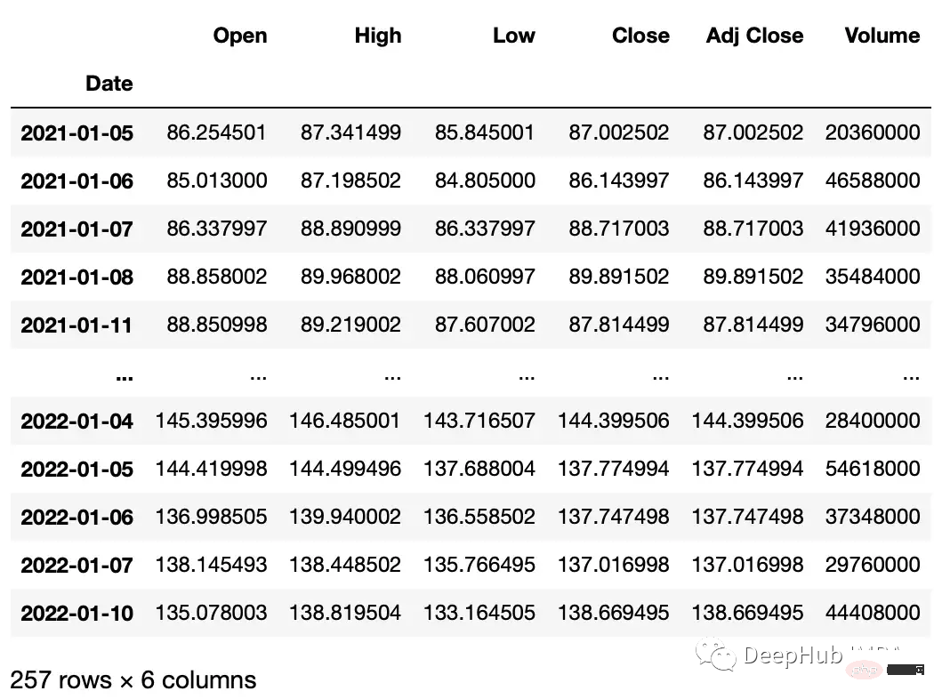
Common data operations
The following is to perform operations on the values in the time series data set. We use the yfinance library to create a stock dataset for our example.
#get google stock price data
import yfinance as yf
start_date = '2020-01-01'
end_date = '2023-01-01'
ticker = 'GOOGL'
df = yf.download(ticker, start_date, end_date)
df.head()

"""
Date Open High Low Close Adj Close Volume
2020-01-02 67.420502 68.433998 67.324501 68.433998 68.433998 27278000
2020-01-03 67.400002 68.687500 67.365997 68.075996 68.075996 23408000
2020-01-06 67.581497 69.916000 67.550003 69.890503 69.890503 46768000
2020-01-07 70.023003 70.175003 69.578003 69.755501 69.755501 34330000
2020-01-08 69.740997 70.592499 69.631500 70.251999 70.251999 35314000
"""
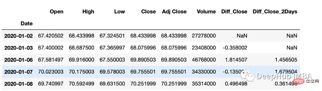
Calculate difference
The diff function can calculate the interpolation between one element and another element.
#subtract that day's value from the previous day
df["Diff_Close"] = df["Close"].diff()
#Subtract that day's value from the day's value 2 days ago
df["Diff_Close_2Days"] = df["Close"].diff(periods=2)
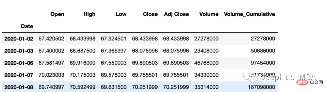
累计总数
df["Volume_Cumulative"] = df["Volume"].cumsum()
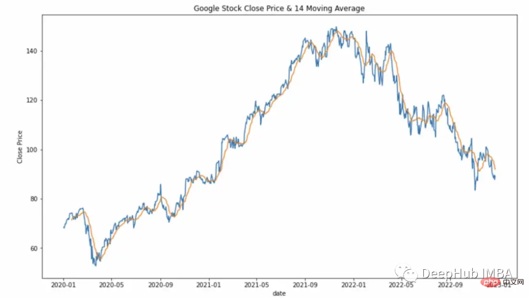
滚动窗口计算
滚动窗口计算(移动平均线)。
df["Close_Rolling_14"] = df["Close"].rolling(14).mean()
df.tail()
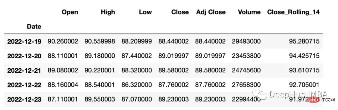
可以对我们计算的移动平均线进行可视化
常用的参数:
- center:决定滚动窗口是否应以当前观测值为中心。
- min_periods:窗口中产生结果所需的最小观测次数。
s = pd.Series([1, 2, 3, 4, 5])

#the rolling window will be centered on each observation
rolling_mean = s.rolling(window=3, center=True).mean()
"""
0 NaN
1 2.0
2 3.0
3 4.0
4 NaN
dtype: float64
Explanation:
first window: [na 1 2] = na
second window: [1 2 3] = 2
"""

# the rolling window will not be centered,
#and will instead be anchored to the left side of the window
rolling_mean = s.rolling(window=3, center=False).mean()
"""
0 NaN
1 NaN
2 2.0
3 3.0
4 4.0
dtype: float64
Explanation:
first window: [na na 1] = na
second window: [na 1 2] = na
third window: [1 2 3] = 2
"""
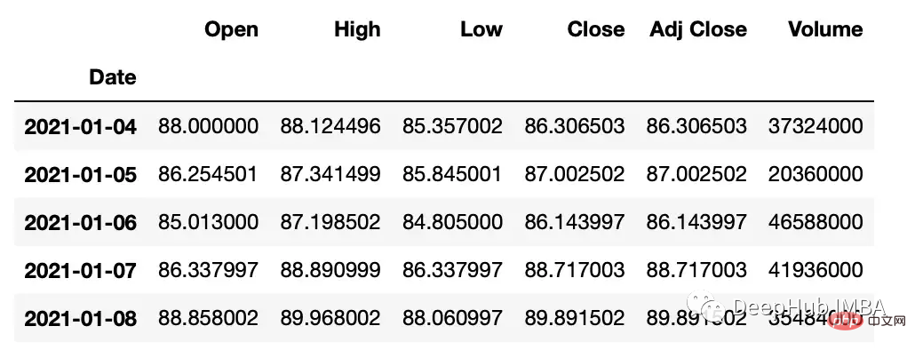
平移
Pandas有两个方法,shift()和tshift(),它们可以指定倍数移动数据或时间序列的索引。Shift()移位数据,而tshift()移位索引。
#shift the data
df_shifted = df.shift(5,axis=0)
df_shifted.head(10)

#shift the indexes
df_tshifted = df.tshift(periods = 4, freq = 'D')
df_tshifted.head(10)
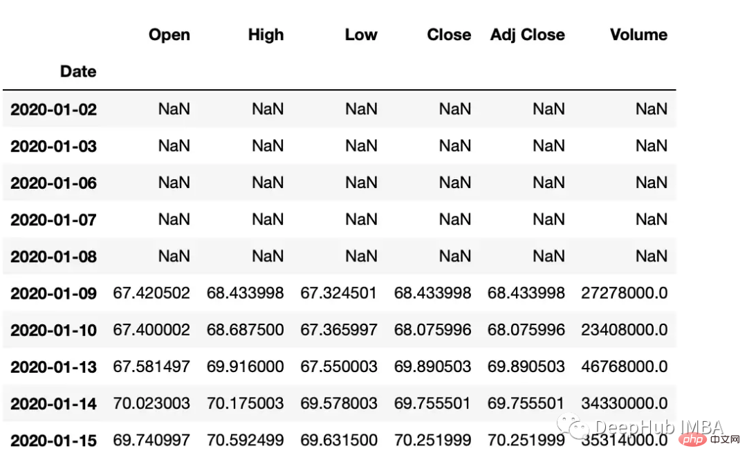
df_shifted
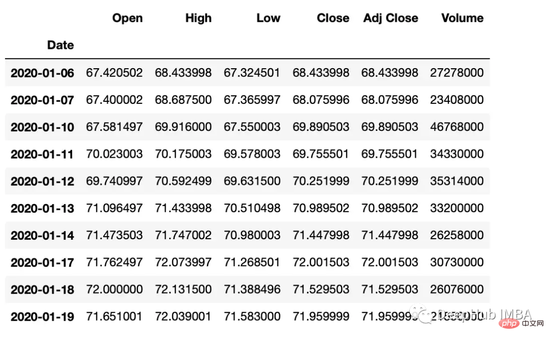
df_tshifted
时间间隔转换
在 Pandas 中,操 to_period 函数允许将日期转换为特定的时间间隔。可以获取具有许多不同间隔或周期的日期
df["Period"] = df["Date"].dt.to_period('W')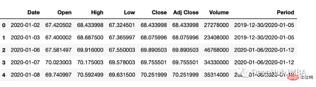
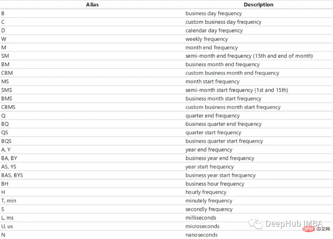
频率
Asfreq方法用于将时间序列转换为指定的频率。
monthly_data = df.asfreq('M', method='ffill')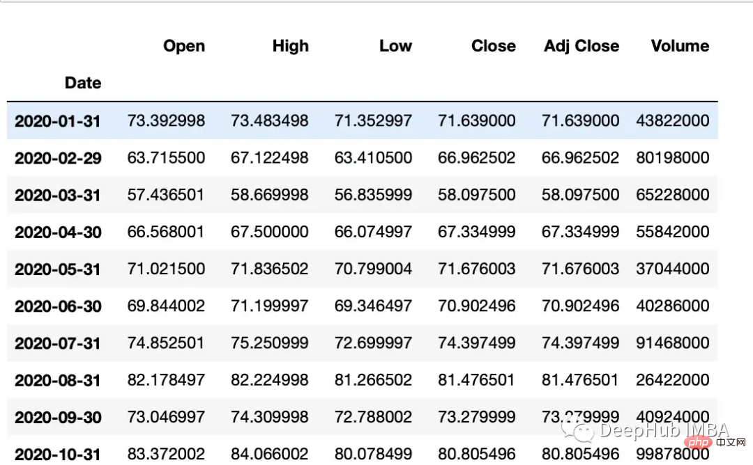
常用参数:
freq:数据应该转换到的频率。这可以使用字符串别名(例如,'M'表示月,'H'表示小时)或pandas偏移量对象来指定。
method:如何在转换频率时填充缺失值。这可以是'ffill'(向前填充)或'bfill'(向后填充)之类的字符串。
采样
resample可以改变时间序列频率并重新采样。我们可以进行上采样(到更高的频率)或下采样(到更低的频率)。因为我们正在改变频率,所以我们需要使用一个聚合函数(比如均值、最大值等)。
resample方法的参数:
rule:数据重新采样的频率。这可以使用字符串别名(例如,'M'表示月,'H'表示小时)或pandas偏移量对象来指定。
#down sample
monthly_data = df.resample('M').mean()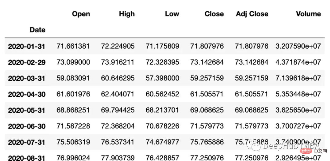
#up sample
minute_data = data.resample('T').ffill()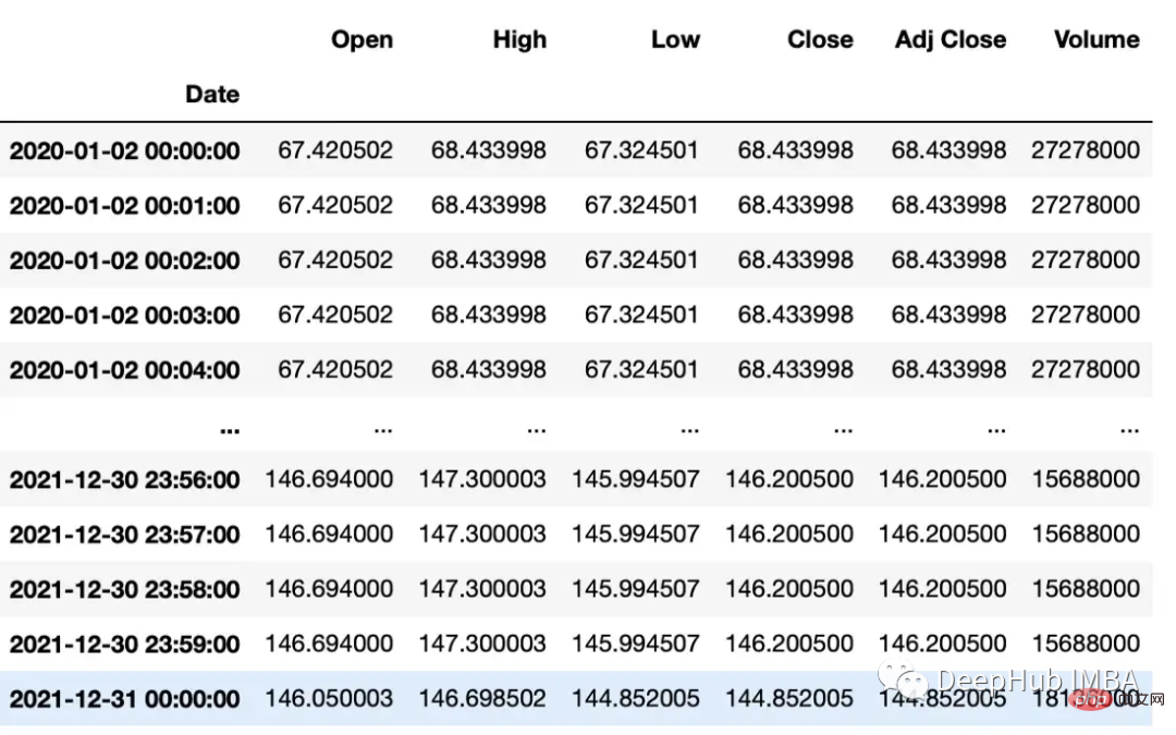
百分比变化
使用pct_change方法来计算日期之间的变化百分比。
df["PCT"] = df["Close"].pct_change(periods=2)
print(df["PCT"])
"""
Date
2020-01-02 NaN
2020-01-03 NaN
2020-01-06 0.021283
2020-01-07 0.024671
2020-01-08 0.005172
...
2022-12-19 -0.026634
2022-12-20 -0.013738
2022-12-21 0.012890
2022-12-22 -0.014154
2022-12-23 -0.003907
Name: PCT, Length: 752, dtype: float64
"""
总结
在Pandas和NumPy等库的帮助下,可以对时间序列数据执行广泛的操作,包括过滤、聚合和转换。本文介绍的是一些在工作中经常遇到的常见操作,希望对你有所帮助。
The above is the detailed content of Summary of common methods for Python time series data manipulation. For more information, please follow other related articles on the PHP Chinese website!

Hot AI Tools

Undress AI Tool
Undress images for free

Undresser.AI Undress
AI-powered app for creating realistic nude photos

AI Clothes Remover
Online AI tool for removing clothes from photos.

Clothoff.io
AI clothes remover

Video Face Swap
Swap faces in any video effortlessly with our completely free AI face swap tool!

Hot Article
Hot Tools

Notepad++7.3.1
Easy-to-use and free code editor

SublimeText3 Chinese version
Chinese version, very easy to use

Zend Studio 13.0.1
Powerful PHP integrated development environment

Dreamweaver CS6
Visual web development tools

SublimeText3 Mac version
God-level code editing software (SublimeText3)


 What are common strategies for debugging a memory leak in Python?
Aug 06, 2025 pm 01:43 PM
What are common strategies for debugging a memory leak in Python?
Aug 06, 2025 pm 01:43 PM
Usetracemalloctotrackmemoryallocationsandidentifyhigh-memorylines;2.Monitorobjectcountswithgcandobjgraphtodetectgrowingobjecttypes;3.Inspectreferencecyclesandlong-livedreferencesusingobjgraph.show_backrefsandcheckforuncollectedcycles;4.Usememory_prof
 What is sentiment analysis in cryptocurrency trading?
Aug 14, 2025 am 11:15 AM
What is sentiment analysis in cryptocurrency trading?
Aug 14, 2025 am 11:15 AM
Table of Contents What is sentiment analysis in cryptocurrency trading? Why sentiment analysis is important in cryptocurrency investment Key sources of emotion data a. Social media platform b. News media c. Tools for sentiment analysis and technology Commonly used tools in sentiment analysis: Techniques adopted: Integrate sentiment analysis into trading strategies How traders use it: Strategy example: Assuming BTC trading scenario scenario setting: Emotional signal: Trader interpretation: Decision: Results: Limitations and risks of sentiment analysis Using emotions for smarter cryptocurrency trading Understanding market sentiment is becoming increasingly important in cryptocurrency trading. A recent 2025 study by Hamid
 How to automate data entry from Excel to a web form with Python?
Aug 12, 2025 am 02:39 AM
How to automate data entry from Excel to a web form with Python?
Aug 12, 2025 am 02:39 AM
The method of filling Excel data into web forms using Python is: first use pandas to read Excel data, and then use Selenium to control the browser to automatically fill and submit the form; the specific steps include installing pandas, openpyxl and Selenium libraries, downloading the corresponding browser driver, using pandas to read Name, Email, Phone and other fields in the data.xlsx file, launching the browser through Selenium to open the target web page, locate the form elements and fill in the data line by line, using WebDriverWait to process dynamic loading content, add exception processing and delay to ensure stability, and finally submit the form and process all data lines in a loop.
 How to use enumerate to loop with an index in Python
Aug 11, 2025 pm 01:14 PM
How to use enumerate to loop with an index in Python
Aug 11, 2025 pm 01:14 PM
When you need to traverse the sequence and access the index, you should use the enumerate() function. 1. enumerate() automatically provides the index and value, which is more concise than range(len(sequence)); 2. You can specify the starting index through the start parameter, such as start=1 to achieve 1-based count; 3. You can use it in combination with conditional logic, such as skipping the first item, limiting the number of loops or formatting the output; 4. Applicable to any iterable objects such as lists, strings, and tuples, and support element unpacking; 5. Improve code readability, avoid manually managing counters, and reduce errors.
 How to implement a custom iterator within a Python class?
Aug 06, 2025 pm 01:17 PM
How to implement a custom iterator within a Python class?
Aug 06, 2025 pm 01:17 PM
Define__iter__()toreturntheiteratorobject,typicallyselforaseparateiteratorinstance.2.Define__next__()toreturnthenextvalueandraiseStopIterationwhenexhausted.Tocreateareusablecustomiterator,managestatewithin__iter__()oruseaseparateiteratorclass,ensurin
 How to copy files and directories from one location to another in Python
Aug 11, 2025 pm 06:11 PM
How to copy files and directories from one location to another in Python
Aug 11, 2025 pm 06:11 PM
To copy files and directories, Python's shutil module provides an efficient and secure approach. 1. Use shutil.copy() or shutil.copy2() to copy a single file, which retains metadata; 2. Use shutil.copytree() to recursively copy the entire directory. The target directory cannot exist in advance, but the target can be allowed to exist through dirs_exist_ok=True (Python3.8); 3. You can filter specific files in combination with ignore parameters and shutil.ignore_patterns() or custom functions; 4. Copying directory only requires os.walk() and os.makedirs()
 How to use Python for stock market analysis and prediction?
Aug 11, 2025 pm 06:56 PM
How to use Python for stock market analysis and prediction?
Aug 11, 2025 pm 06:56 PM
Python can be used for stock market analysis and prediction. The answer is yes. By using libraries such as yfinance, using pandas for data cleaning and feature engineering, combining matplotlib or seaborn for visual analysis, then using models such as ARIMA, random forest, XGBoost or LSTM to build a prediction system, and evaluating performance through backtesting. Finally, the application can be deployed with Flask or FastAPI, but attention should be paid to the uncertainty of market forecasts, overfitting risks and transaction costs, and success depends on data quality, model design and reasonable expectations.
 How to handle large datasets in Python that don't fit into memory?
Aug 14, 2025 pm 01:00 PM
How to handle large datasets in Python that don't fit into memory?
Aug 14, 2025 pm 01:00 PM
When processing large data sets that exceed memory in Python, they cannot be loaded into RAM at one time. Instead, strategies such as chunking processing, disk storage or streaming should be adopted; CSV files can be read in chunks through Pandas' chunksize parameters and processed block by block. Dask can be used to realize parallelization and task scheduling similar to Pandas syntax to support large memory data operations. Write generator functions to read text files line by line to reduce memory usage. Use Parquet columnar storage format combined with PyArrow to efficiently read specific columns or row groups. Use NumPy's memmap to memory map large numerical arrays to access data fragments on demand, or store data in lightweight data such as SQLite or DuckDB.
