An in-depth discussion of 2D and 3D visual perception algorithms in autonomous driving

Environmental perception is the first link in autonomous driving and the link between the vehicle and the environment. The overall performance of an autonomous driving system largely depends on the quality of the perception system. At present, there are two mainstream technology routes for environmental perception technology:

① Vision-led multi-sensor fusion solution, the typical representative is Tesla;

② Lidar-led, other Sensor-assisted technical solutions, typical representatives such as Google, Baidu, etc.

We will introduce the key visual perception algorithms in environmental perception. Its task coverage and its technical fields are shown in the figure below. We review the context and direction of 2D and 3D visual perception algorithms below.

2D visual perception

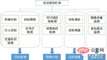
In this section, we first introduce the 2D visual perception algorithm starting from several tasks that are widely used in autonomous driving. , including image or video-based 2D object detection and tracking, and semantic segmentation of 2D scenes. In recent years, deep learning has penetrated into various fields of visual perception and achieved good results. Therefore, we have sorted out some classic deep learning algorithms.

1. Target detection

1.1 Two-stage detection

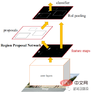
The two-stage refers to the two ways to achieve detection. There are two processes, one is to extract the object area; the other is to classify and identify the area with CNN; therefore, the "two-stage" is also called target detection based on the candidate region (Region proposal). Representative algorithms include the R-CNN series (R-CNN, Fast R-CNN, Faster R-CNN), etc. Faster R-CNN is the first end-to-end detection network. In the first stage, a region candidate network (RPN) is used to generate candidate frames based on the feature map, and ROIPooling is used to align the size of the candidate features; in the second stage, a fully connected layer is used for refined classification and regression.

The idea of ​​Anchor is proposed here to reduce the difficulty of calculation and increase the speed. Each position of the feature map will generate Anchors of different sizes and aspect ratios, which are used as a reference for object frame regression. The introduction of Anchor allows the regression task to only deal with relatively small changes, so the network learning will be easier. The figure below is the network structure diagram of Faster R-CNN.

The first stage of CascadeRCNN is exactly the same as Faster R-CNN, and the second stage uses multiple RoiHead layers for cascading. The subsequent work mostly revolves around some improvements of the above-mentioned network or a hodgepodge of previous work, with few breakthrough improvements.

1.2 Single-stage detection

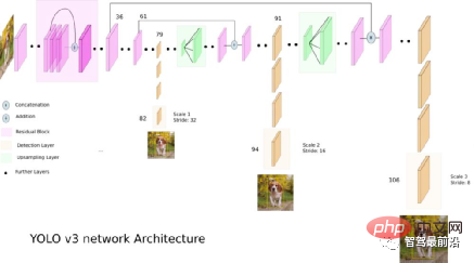
Compared with the two-stage algorithm, the single-stage algorithm only needs to extract features once to achieve target detection. Its speed algorithm is faster and generally The accuracy is slightly lower. The pioneering work of this type of algorithm is YOLO, which was subsequently improved by SSD and Retinanet. The team that proposed YOLO integrated these tricks that help improve performance into the YOLO algorithm, and subsequently proposed 4 improved versions YOLOv2~ YOLOv5. Although the prediction accuracy is not as good as the two-stage target detection algorithm, YOLO has become the mainstream in the industry due to its faster running speed. The figure below is the network structure diagram of YOLO v3.

1.3 Anchor-free detection (no Anchor detection)

This type of method generally represents the object as some key points. CNN is used to return the locations of these key points. The key point can be the center point (CenterNet), corner point (CornerNet) or representative point (RepPoints) of the object frame. CenterNet converts the target detection problem into a center point prediction problem, that is, using the center point of the target to represent the target, and obtaining the rectangular frame of the target by predicting the offset, width and height of the target center point. Heatmap represents classification information, and each category will generate a separate Heatmap. For each Heatmap, when a certain coordinate contains the center point of the target, a key point will be generated at the target. We use a Gaussian circle to represent the entire key point. The following figure shows the specific details.

RepPoints proposes to represent the object as a representative point set and adapt to the shape changes of the object through deformable convolution. The point set is finally converted into an object frame and used to calculate the difference from manual annotation.

1.4 Transformer detection

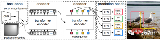
Whether it is single-stage or two-stage target detection, whether Anchor is used or not, the attention mechanism is not well utilized. In response to this situation, Relation Net and DETR use Transformer to introduce the attention mechanism into the field of target detection. Relation Net uses Transformer to model the relationship between different targets, incorporates relationship information into features, and achieves feature enhancement. DETR proposes a new target detection architecture based on Transformer, opening a new era of target detection. The following figure is the algorithm process of DETR. First, CNN is used to extract image features, and then Transformer is used to model the global spatial relationship. Finally, we get The output of is matched with manual annotation through a bipartite graph matching algorithm.

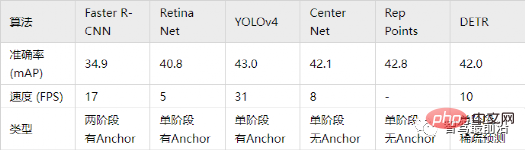
The accuracy in the table below uses mAP on the MS COCO database as an indicator, while the speed is measured by FPS. Compared with some of the above algorithms, due to the structural design of the network There are many different choices (such as different input sizes, different Backbone networks, etc.), and the implementation hardware platforms of each algorithm are also different, so the accuracy and speed are not completely comparable. Here is only a rough result for your reference. .

2. Target tracking

In autonomous driving applications, the input is video data, and there are many targets that need to be paid attention to. Such as vehicles, pedestrians, bicycles, etc. Therefore, this is a typical multiple object tracking task (MOT). For the MOT task, the most popular framework currently is Tracking-by-Detection, and its process is as follows:

① The target detector obtains the target frame output on a single frame image;

② Extract the features of each detected target, usually including visual features and motion features;

③Calculate the similarity between target detections from adjacent frames based on the features to determine the probability that they come from the same target;

④ Match the target detections in adjacent frames and assign the same ID to objects from the same target.

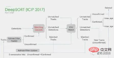
Deep learning is applied in the above four steps, but the first two steps are the main ones. In step 1, the application of deep learning is mainly to provide high-quality object detectors, so methods with higher accuracy are generally chosen. SORT is a target detection method based on Faster R-CNN, and uses the Kalman filter algorithm Hungarian algorithm to greatly improve the speed of multi-target tracking and achieve the accuracy of SOTA. It is also an algorithm widely used in practical applications. . In step 2, the application of deep learning mainly relies on using CNN to extract the visual features of objects. The biggest feature of DeepSORT is to add appearance information and borrow the ReID module to extract deep learning features, reducing the number of ID switches. The overall flow chart is as follows:

#In addition, there is also a framework Simultaneous Detection and Tracking. Such as the representative CenterTrack, which originated from the single-stage Anchor-less detection algorithm CenterNet introduced before. Compared with CenterNet, CenterTrack adds the RGB image of the previous frame and the object center Heatmap as additional inputs, and adds an Offset branch for association between the previous and next frames. Compared with multi-stage Tracking-by-Detection, CenterTrack uses a network to implement the detection and matching stages, which improves the speed of MOT.

3. Semantic segmentation

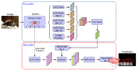
Semantic segmentation is used in both the lane line detection and drivable area detection tasks of autonomous driving. Representative algorithms include FCN, U-Net, DeepLab series, etc. DeepLab uses dilated convolution and ASPP (Atrous Spatial Pyramid Pooling) structure to perform multi-scale processing on the input image. Finally, the conditional random field (CRF) commonly used in traditional semantic segmentation methods is used to optimize the segmentation results. The figure below is the network structure of DeepLab v3.

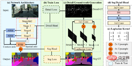
#The STDC algorithm in recent years adopts a structure similar to the FCN algorithm, removing the complex decoder structure of the U-Net algorithm. But at the same time, in the process of network downsampling, the ARM module is used to continuously fuse information from different layer feature maps, thus avoiding the shortcoming of the FCN algorithm that only considers the relationship of a single pixel. It can be said that the STDC algorithm achieves a good balance between speed and accuracy, and it can meet the real-time requirements of the autonomous driving system. The algorithm flow is shown in the figure below.

3D visual perception

In this section we will introduce the 3D scene perception that is essential in autonomous driving. Because depth information, target three-dimensional size, etc. cannot be obtained in 2D perception, and this information is the key for the autonomous driving system to make correct judgments on the surrounding environment. The most direct way to obtain 3D information is to use LiDAR. However, LiDAR also has its shortcomings, such as higher cost, difficulty in mass production of automotive-grade products, greater impact from weather, etc. Therefore, 3D perception based solely on cameras is still a very meaningful and valuable research direction. Next, we sort out some 3D perception algorithms based on monocular and binocular.

1. Monocular 3D perception

Perceiving the 3D environment based on a single camera image is an ill-posed problem, but it can be made through geometric assumptions (such as pixels on the ground), Prior knowledge or some additional information (such as depth estimation) to assist in solving. This time we will introduce the relevant algorithms starting from the two basic tasks of realizing autonomous driving (3D target detection and depth estimation).

1.1 3D target detection

#Representation conversion (pseudo lidar): The detection of other surrounding vehicles by visual sensors usually When encountering problems such as occlusion and inability to measure distances, the perspective view can be converted into a bird's-eye view representation. Two transformation methods are introduced here. The first is inverse perspective mapping (IPM), which assumes that all pixels are on the ground and the camera external parameters are accurate. At this time, Homography transformation can be used to convert the image to BEV, and then a method based on the YOLO network is used to detect the ground frame of the target. . The second is Orthogonal Feature Transform (OFT), which uses ResNet-18 to extract perspective image features. Voxel-based features are then generated by accumulating image-based features over the projected voxel regions.

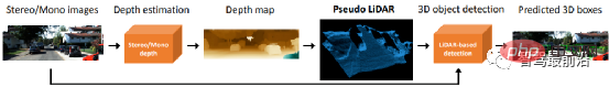
The voxel features are then folded vertically to produce orthogonal ground plane features. Finally, another top-down network similar to ResNet is used for 3D object detection. These methods are only suitable for vehicles and pedestrians that are close to the ground. For non-ground targets such as traffic signs and traffic lights, pseudo point clouds can be generated through depth estimation for 3D detection. Pseudo-LiDAR first uses the depth estimation results to generate point clouds, and then directly applies the lidar-based 3D target detector to generate a 3D target frame. The algorithm flow is shown in the figure below,

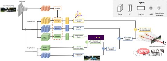
Key points and 3D models: The size and shape of the targets to be detected, such as vehicles and pedestrians, are relatively fixed and known. These can be used as prior knowledge to estimate the 3D information of the targets. DeepMANTA is one of the pioneering works in this direction. First, some target detection algorithms such as Faster RNN are used to obtain the 2D target frame and also detect the key points of the target. Then, these 2D target frames and key points are matched with various 3D vehicle CAD models in the database, and the model with the highest similarity is selected as the output of 3D target detection. MonoGRNet proposes to divide monocular 3D target detection into four steps: 2D target detection, instance-level depth estimation, projected 3D center estimation and local corner regression. The algorithm flow is shown in the figure below. This type of method assumes that the target has a relatively fixed shape model, which is generally satisfactory for vehicles, but is relatively difficult for pedestrians.

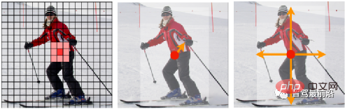
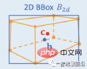
2D/3D Geometric Constraints: Regress the projection of the 3D center and rough instance depth and use both to estimate a rough 3D position. The pioneering work is Deep3DBox, which first uses image features within a 2D target box to estimate target size and orientation. Then, the 3D position of the center point is solved through a 2D/3D geometric constraint. This constraint is that the projection of the 3D target frame on the image is closely surrounded by the 2D target frame, that is, at least one corner point of the 3D target frame can be found on each side of the 2D target frame. Through the previously predicted size and orientation, combined with the camera's calibration parameters, the 3D position of the center point can be calculated. The geometric constraints between the 2D and 3D target boxes are shown in the figure below. Based on Deep3DBox, Shift R-CNN combines the previously obtained 2D target box, 3D target box and camera parameters as input, and uses a fully connected network to predict a more accurate 3D position.

Directly generate 3DBox: This method starts from dense 3D target candidate boxes and scores all candidate boxes based on the features on the 2D image. The candidate box with a high score is the final output. Somewhat similar to the traditional sliding window method in target detection. The representative Mono3D algorithm first generates dense 3D candidate boxes based on the target's prior position (z coordinate is on the ground) and size. After these 3D candidate frames are projected to image coordinates, they are scored by integrating the features on the 2D image, and then a second round of scoring is performed through CNN to obtain the final 3D target frame.

M3D-RPN is an Anchor-based method that defines 2D and 3D Anchors. The 2D Anchor is obtained through dense sampling on the image, and the 3D Anchor is determined through the prior knowledge of the training set data (such as the mean of the actual size of the target). M3D-RPN also uses both standard convolution and Depth-Aware convolution. The former has spatial invariance, and the latter divides the rows (Y coordinates) of the image into multiple groups. Each group corresponds to a different scene depth and is processed by different convolution kernels. The above dense sampling methods are very computationally intensive. SS3D uses a more efficient single-stage detection, including a CNN for outputting redundant representations of each relevant object in the image and corresponding uncertainty estimates, and a 3D bounding box optimizer. FCOS3D is also a single-stage detection method. The regression target adds an additional 2.5D center (X, Y, Depth) obtained by projecting the center of the 3D target frame onto the 2D image.

1.2 Depth Estimation

Whether it is the above-mentioned 3D target detection or another important task of autonomous driving perception-semantic segmentation, extending from 2D to 3D, More or less sparse or dense depth information is applied. The importance of monocular depth estimation is self-evident. Its input is an image, and the output is an image of the same size consisting of the scene depth value corresponding to each pixel. The input can also be a video sequence, using additional information brought by camera or object motion to improve the accuracy of depth estimation. Compared with supervised learning, the unsupervised method of monocular depth estimation does not require the construction of a challenging ground truth data set and is less difficult to implement. Unsupervised methods for monocular depth estimation can be divided into two types: based on monocular video sequences and based on synchronized stereo image pairs.

The former is based on the assumption of moving cameras and static scenes. In the latter method, Garg et al. first tried to use stereo-corrected binocular image pairs at the same moment for image reconstruction. The pose relationship between the left and right views was obtained through binocular determination, and a relatively ideal effect was achieved. On this basis, Godard et al. used left and right consistency constraints to further improve the accuracy. However, while extracting advanced features through layer-by-layer downsampling to increase the receptive field, the feature resolution is also constantly declining, and the granularity is constantly lost, affecting Deep detail processing and edge clarity.

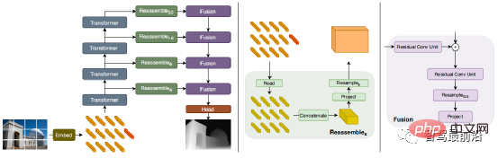
To alleviate this problem, Godard et al. introduced a full-resolution multi-scale loss, which effectively reduced black holes and texture replication artifacts in low-texture areas. However, this improvement in accuracy is still limited. Recently, some Transformer-based models have emerged in an endless stream, aiming to obtain a global receptive field in all stages, which is also very suitable for intensive depth estimation tasks. In supervised DPT, it is proposed to use Transformer and multi-scale structure to simultaneously ensure the local accuracy and global consistency of prediction. The following figure is the network structure diagram.

2. Binocular 3D perception

Binocular vision can solve the ambiguity caused by perspective transformation, so theoretically It is said that it can improve the accuracy of 3D perception. However, the binocular system has relatively high requirements in terms of hardware and software. In terms of hardware, two accurately registered cameras are required, and the accuracy of the registration must be ensured during vehicle operation. In terms of software, the algorithm needs to process data from two cameras at the same time. The calculation complexity is high, and the real-time performance of the algorithm is difficult to guarantee. Compared to monocular, binocular work is relatively less. Next, we will also give a brief introduction from the two aspects of 3D target detection and depth estimation.

2.1 3D target detection

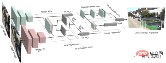
3DOP is a two-stage detection method and an expansion of the Fast R-CNN method in the 3D field. First, binocular images are used to generate a depth map. The depth map is converted into a point cloud and then quantified into a grid data structure. This is then used as input to generate a candidate frame for the 3D target. Similar to the Pseudo-LiDAR introduced before, dense depth maps (from monocular, binocular or even low-line-number LiDAR) are converted into point clouds, and then algorithms in the field of point cloud target detection are applied. DSGN utilizes stereo matching to construct planar scan volumes and converts them into 3D geometry in order to encode 3D geometry and semantic information. It is an end-to-end framework that can extract pixel-level features for stereo matching and advanced object recognition. features, and can simultaneously estimate scene depth and detect 3D objects. Stereo R-CNN extends Faster R-CNN for stereo input to detect and correlate objects in left and right views simultaneously. An additional branch is added after RPN to predict sparse keypoints, viewpoints and object sizes, and combines the 2D bounding boxes in the left and right views to calculate a coarse 3D object bounding box. Then, accurate 3D bounding boxes are recovered by using region-based photometric alignment of the left and right regions of interest. The figure below is its network structure.

2.2 Depth estimation

The principle of binocular depth estimation is very simple, that is, based on the distance between the same 3D points on the left and right views The pixel distance d (assuming the two cameras remain at the same height, so only the distance in the horizontal direction is considered), that is, the disparity, the focal length f of the camera, and the distance B (baseline length) between the two cameras, to estimate the depth of the 3D point, The formula is as follows, and the depth can be calculated by estimating the parallax. Then, all you need to do is find a matching point on the other image for each pixel.

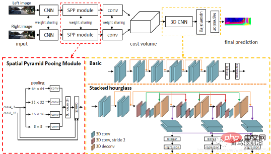
For each possible d, the matching error at each pixel can be calculated, so a three-dimensional error data Cost Volume is obtained. Through Cost Volume, we can easily get the disparity at each pixel (d corresponding to the minimum matching error), and thus obtain the depth value. MC-CNN uses a convolutional neural network to predict the matching degree of two image patches and uses it to calculate the stereo matching cost. Costs are refined through intersection-based cost aggregation and semi-global matching, followed by left-right consistency checks to eliminate errors in occluded areas. PSMNet proposes an end-to-end learning framework for stereo matching that does not require any post-processing, introduces a pyramid pooling module to incorporate global context information into image features, and provides a stacked hourglass 3D CNN to further enhance global information. The figure below is its network structure.

The above is the detailed content of An in-depth discussion of 2D and 3D visual perception algorithms in autonomous driving. For more information, please follow other related articles on the PHP Chinese website!