Theory, implementation and hyperparameter tuning of decision trees and random forests

In this article, we will introduce the decision tree and random forest models in detail. Furthermore, we will show which hyperparameters of decision trees and random forests have a significant impact on their performance, allowing us to find the optimal solution between underfitting and overfitting. After understanding the theory behind decision trees and random forests. , we will implement them using Scikit-Learn.

1. Decision tree

Decision tree is an important algorithm for predictive modeling machine learning. The classic decision tree algorithm has been around for decades, and modern variants like random forests are among the most powerful techniques available.

Typically, such algorithms are called "decision trees", but on some platforms such as R, they are called CART. The CART algorithm provides the basis for important algorithms such as bagged decision trees, random forests, and boosting decision trees.

Unlike linear models, decision trees are non-parametric models: they are not controlled by a mathematical decision function and have no weights or intercepts to optimize. In effect, a decision tree will divide the space by taking features into account.

CART model representation

The representation of the CART model is a binary tree. This is a binary tree from algorithms and data structures. Each root node represents an input variable (x) and a split point on that variable (assuming the variable is numeric).

The leaf nodes of the tree contain an output variable (y), which is used to make predictions. Given a new input, the tree is traversed by computing the specific input starting from the root node of the tree.

Some advantages of decision trees are:

• Easy to understand and interpret. Trees can be visualized.
• Requires little data preparation.
• Ability to handle numerical and categorical data.
• Statistical tests can be used to validate the model.
• Perform well even if the real model that generated the data violates its assumptions to some extent.

Disadvantages of decision trees include:

• Overfitting. Mechanisms such as pruning, setting the minimum number of samples required for leaf nodes, or setting the maximum depth of the tree are necessary to avoid this problem.
• Decision trees may be unstable. Decision trees can be used in ensembles.
• There is no guarantee that the global optimal decision tree will be returned. Multiple trees can be trained in one ensemble learner
• Decision tree learners create biased trees if certain categories dominate. Recommendation: Balance the data set before fitting

2. Random Forest

Random Forest is one of the most popular and powerful machine learning algorithms. It is an integrated machine learning algorithm called Bootstrap Aggregation or bagging.

To improve the performance of decision trees, we can use many trees with random feature samples.

3.Decision tree and random forest implementation in python

We will use decision tree and random forest to predict the loss of your valuable employees.

import pandas as pd
import numpy as np
import matplotlib.pyplot as plt
import seaborn as sns
%matplotlib inline


sns.set_style("whitegrid")
plt.style.use("fivethirtyeight")
df = pd.read_csv("WA_Fn-UseC_-HR-Employee-Attrition.csv")

from sklearn.preprocessing import LabelEncoder
from sklearn.model_selection import train_test_split




df.drop(['EmployeeCount', 'EmployeeNumber', 'Over18', 'StandardHours'], axis="columns", inplace=True)


categorical_col = []
for column in df.columns:
if df[column].dtype == object and len(df[column].unique())  50:
categorical_col.append(column)
df['Attrition'] = df.Attrition.astype("category").cat.codes


categorical_col.remove('Attrition')


label = LabelEncoder()
for column in categorical_col:
df[column] = label.fit_transform(df[column])


X = df.drop('Attrition', axis=1)
y = df.Attrition


X_train, X_test, y_train, y_test = train_test_split(X, y, test_size=0.3, random_state=42)

Copy after login

from sklearn.metrics import accuracy_score, confusion_matrix, classification_report


def print_score(clf, X_train, y_train, X_test, y_test, train=True):
if train:
pred = clf.predict(X_train)
print("Train Result:n================================================")
print(f"Accuracy Score: {accuracy_score(y_train, pred) * 100:.2f}%")
print("_______________________________________________")
print(f"Confusion Matrix: n {confusion_matrix(y_train, pred)}n")
elif train==False:
pred = clf.predict(X_test)
print("Test Result:n================================================")
print(f"Accuracy Score: {accuracy_score(y_test, pred) * 100:.2f}%")
print("_______________________________________________")
print(f"Confusion Matrix: n {confusion_matrix(y_test, pred)}n")

Copy after login

criterion: Measures split quality. Supported criteria are "Gini" for impurity and "Entropy" for information gain.
• splitter: The strategy used to select splits at each node. Supported strategies are "best" which selects the best split and "random" which selects a random split.
• max_depth: The maximum depth of the tree. If None, expand nodes until all leaf nodes, or until all leaves contain less than min_samples_split samples.
• min_samples_split: The minimum number of samples required to split internal nodes.
• min_samples_leaf: The minimum number of samples required on leaf nodes.
• min_weight_fraction_leaf: The minimum weighted fraction of the total weight required on the leaf node. When sample_weight is not provided, samples have equal weight.
• max_features: The number of features to consider when finding the best split.
• max_leaf_nodesmax_leaf_nodes: Use max_leaf_nodes to form the tree in a best-first manner. The optimal node is defined as the relative reduction of impurities. If None, there are an unlimited number of leaf nodes.
• min_impurity_decrease: If the split results in an impurity reduction greater than or equal to this value, the node will be split.
• min_impurity_split: Threshold for early stopping. If the impurity of a node is above the threshold, the node is split, otherwise, it is a leaf.

from sklearn.tree import DecisionTreeClassifier


tree_clf = DecisionTreeClassifier(random_state=42)
tree_clf.fit(X_train, y_train)


print_score(tree_clf, X_train, y_train, X_test, y_test, train=True)
print_score(tree_clf, X_train, y_train, X_test, y_test, train=False)

from sklearn.tree import DecisionTreeClassifier
from sklearn.model_selection import GridSearchCV


params = {
"criterion":("gini", "entropy"), 
"splitter":("best", "random"), 
"max_depth":(list(range(1, 20))), 
"min_samples_split":[2, 3, 4], 
"min_samples_leaf":list(range(1, 20)), 
}


tree_clf = DecisionTreeClassifier(random_state=42)
tree_cv = GridSearchCV(tree_clf, params, scoring="accuracy", n_jobs=-1, verbose=1, cv=3)
tree_cv.fit(X_train, y_train)
best_params = tree_cv.best_params_
print(f"Best paramters: {best_params})")


tree_clf = DecisionTreeClassifier(**best_params)
tree_clf.fit(X_train, y_train)
print_score(tree_clf, X_train, y_train, X_test, y_test, train=True)
print_score(tree_clf, X_train, y_train, X_test, y_test, train=False)

5.3树的可视化

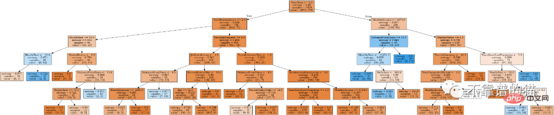
from IPython.display import Image
from six import StringIO
from sklearn.tree import export_graphviz
import pydot


features = list(df.columns)
features.remove("Attrition")
dot_data = StringIO()
export_graphviz(tree_clf, out_file=dot_data, feature_names=features, filled=True)
graph = pydot.graph_from_dot_data(dot_data.getvalue())
Image(graph[0].create_png())

5.4随机森林

随机森林是一种元估计器，它将多个决策树分类器对数据集的不同子样本进行拟合，并使用均值来提高预测准确度和控制过拟合。

随机森林算法参数:

• n_estimators: 树的数量。
• criterion: 衡量拆分质量的函数。支持的标准是gini和信息增益的“熵”。
• max_depth：树的最大深度。如果为None，则展开节点，直到所有叶子都是纯的，或者直到所有叶子包含的样本少于min_samples_split。
• min_samples_split：拆分内部节点所需的最小样本数。
• min_samples_leaf：叶节点所需的最小样本数。min_samples_leaf只有在左右分支中的每个分支中至少留下训练样本时，才会考虑任何深度的分割点。这可能具有平滑模型的效果，尤其是在回归中。
• min_weight_fraction_leaf：需要在叶节点处的总权重（所有输入样本的）的最小加权分数。当未提供 sample_weight 时，样本具有相同的权重。
• max_features：寻找最佳分割时要考虑的特征数量。
• max_leaf_nodesmax_leaf_nodes：以最佳优先方式种植一棵树。最佳节点定义为杂质的相对减少。如果 None 则无限数量的叶节点。
• min_impurity_decrease：如果该分裂导致杂质减少大于或等于该值，则该节点将被分裂。
• min_impurity_split: 树提前停止的阈值。如果一个节点的杂质高于阈值，则该节点将分裂，否则，它是一个叶子。
• bootstrap：构建树时是否使用bootstrap样本。如果为 False，则使用整个数据集来构建每棵树。
• oob_score：是否使用out-of-bag样本来估计泛化准确度。

from sklearn.ensemble import RandomForestClassifier


rf_clf = RandomForestClassifier(n_estimators=100)
rf_clf.fit(X_train, y_train)


print_score(rf_clf, X_train, y_train, X_test, y_test, train=True)
print_score(rf_clf, X_train, y_train, X_test, y_test, train=False)

5.5随机森林超参数调优

调优随机森林的主要参数是n_estimators参数。一般来说，森林中的树越多，泛化性能越好，但它会减慢拟合和预测的时间。

我们还可以调优控制森林中每棵树深度的参数。有两个参数非常重要:max_depth和max_leaf_nodes。实际上，max_depth将强制具有更对称的树，而max_leaf_nodes会限制最大叶节点数量。

n_estimators = [100, 500, 1000, 1500]
max_features = ['auto', 'sqrt']
max_depth = [2, 3, 5]
max_depth.append(None)
min_samples_split = [2, 5, 10]
min_samples_leaf = [1, 2, 4, 10]
bootstrap = [True, False]


params_grid = {'n_estimators': n_estimators, 'max_features': max_features,
 'max_depth': max_depth, 'min_samples_split': min_samples_split,
 'min_samples_leaf': min_samples_leaf, 'bootstrap': bootstrap}


rf_clf = RandomForestClassifier(random_state=42)


rf_cv = GridSearchCV(rf_clf, params_grid, scoring="f1", cv=3, verbose=2, n_jobs=-1)


rf_cv.fit(X_train, y_train)
best_params = rf_cv.best_params_
print(f"Best parameters: {best_params}")


rf_clf = RandomForestClassifier(**best_params)
rf_clf.fit(X_train, y_train)


print_score(rf_clf, X_train, y_train, X_test, y_test, train=True)
print_score(rf_clf, X_train, y_train, X_test, y_test, train=False)

最后

本文主要讲解了以下内容：

• 决策树和随机森林算法以及每种算法的参数。
• 如何调整决策树和随机森林的超参数。
• 在训练之前需要平衡你的数据集。
• 从每个类中抽取相同数量的样本。
• 通过将每个类的样本权重(sample_weight)的和归一化为相同的值。

The above is the detailed content of Theory, implementation and hyperparameter tuning of decision trees and random forests. For more information, please follow other related articles on the PHP Chinese website!