Step-by-step visualization of the decision-making process of the gradient boosting algorithm

The gradient boosting algorithm is one of the most commonly used ensemble machine learning techniques. This model uses a sequence of weak decision trees to build a strong learner. This is also the theoretical basis of the XGBoost and LightGBM models, so in this article, we will build a gradient boosting model from scratch and visualize it.

Introduction to Gradient Boosting Algorithm

Gradient Boosting algorithm (Gradient Boosting) is an ensemble learning algorithm that improves performance by building multiple weak classifiers and then combining them into a strong classifier. The prediction accuracy of the model.

The principle of gradient boosting algorithm can be divided into the following steps:

1. Initialize the model: Generally speaking, we can use a simple model (such as a decision tree) as the initial classifier.
2. Calculate the negative gradient of the loss function: Calculate the negative gradient of the loss function for each sample point under the current model. This is equivalent to asking the new classifier to fit the error under the current model.
3. Train a new classifier: Use these negative gradients as target variables to train a new weak classifier. This weak classifier can be any classifier, such as decision tree, linear model, etc.
4. Update model: Add new classifiers to the original model, and combine them using weighted average or other methods.
5. Repeat iteration: Repeat the above steps until the preset number of iterations is reached or the preset accuracy is reached.

Since the gradient boosting algorithm is a serial algorithm, its training speed may be slower. Let’s introduce it with a practical example:

Assume we have a feature Set Xi and value Yi, to calculate the best estimate of y

We start with the mean of y

import numpy as np
 import sklearn.datasets as ds
 import pandas as pd
 import matplotlib.pyplot as plt
 import matplotlib as mpl
 
 from sklearn import tree
 from itertools import product,islice
 import seaborn as snsmoonDS = ds.make_moons(200, noise = 0.15, random_state=16)
 moon = moonDS[0]
 color = -1*(moonDS[1]*2-1)
 
 df =pd.DataFrame(moon, columns = ['x','y'])
 df['z'] = color
 df['f0'] =df.y.mean()
 df['r0'] = df['z'] - df['f0']
 df.head(10)

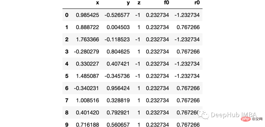
下图可以看到，该数据集是可以明显的区分出分类的边界的，但是因为他是非线性的，所以使用线性算法进行分类时会遇到很大的困难。

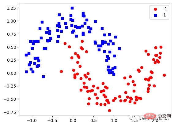
那么我们先编写一个简单的梯度增强模型:

def makeiteration(i:int):
"""Takes the dataframe ith f_i and r_i and approximated r_i from the features, then computes f_i+1 and r_i+1"""
clf = tree.DecisionTreeRegressor(max_depth=1)
clf.fit(X=df[['x','y']].values, y = df[f'r{i-1}'])
df[f'r{i-1}hat'] = clf.predict(df[['x','y']].values)
 
eta = 0.9
df[f'f{i}'] = df[f'f{i-1}'] + eta*df[f'r{i-1}hat']
df[f'r{i}'] = df['z'] - df[f'f{i}']
rmse = (df[f'r{i}']**2).sum()
clfs.append(clf)
rmses.append(rmse)

上面代码执行3个简单步骤:

将决策树与残差进行拟合:

clf.fit(X=df[['x','y']].values, y = df[f'r{i-1}'])
 df[f'r{i-1}hat'] = clf.predict(df[['x','y']].values)

然后，我们将这个近似的梯度与之前的学习器相加:

df[f'f{i}'] = df[f'f{i-1}'] + eta*df[f'r{i-1}hat']

最后重新计算残差:

df[f'r{i}'] = df['z'] - df[f'f{i}']

步骤就是这样简单，下面我们来一步一步执行这个过程。

第1次决策

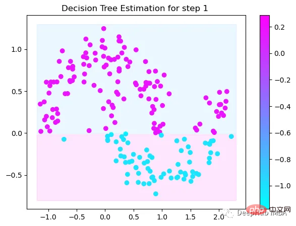
Tree Split for 0 and level 1.563690960407257

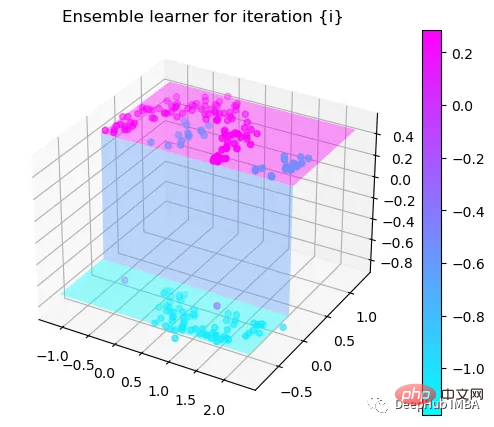
第2次决策

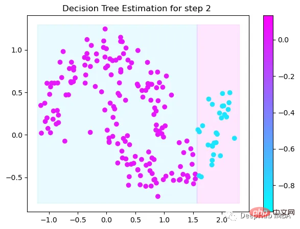
Tree Split for 1 and level 0.5143677890300751

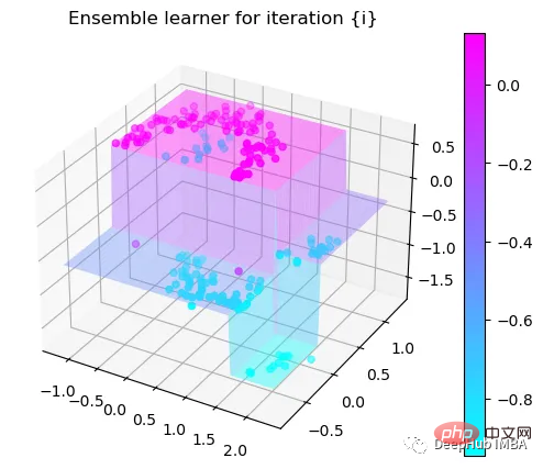
第3次决策

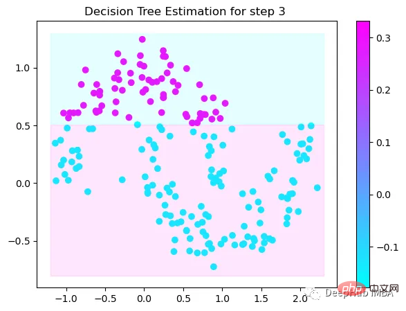
Tree Split for 0 and level -0.6523728966712952

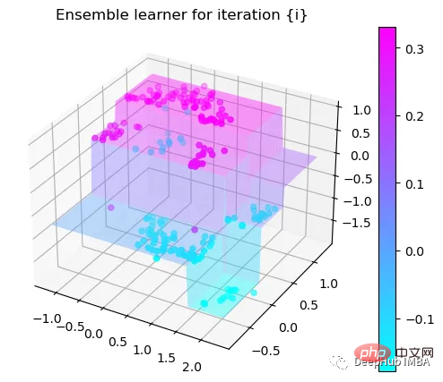
第4次决策

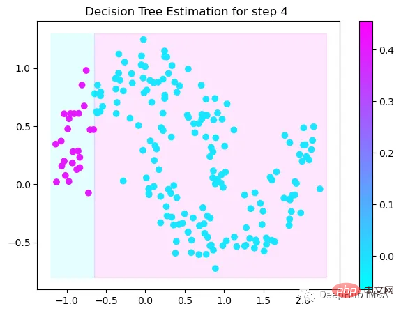
Tree Split for 0 and level 0.3370491564273834

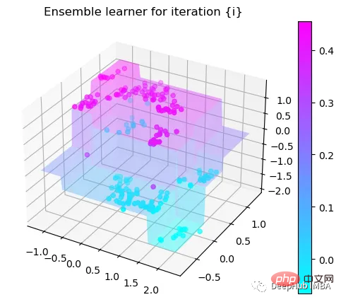
第5次决策

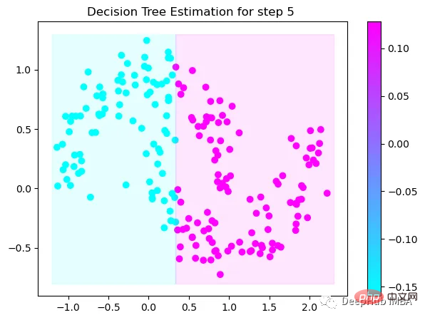
Tree Split for 0 and level 0.3370491564273834

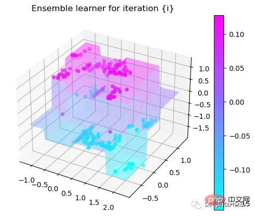
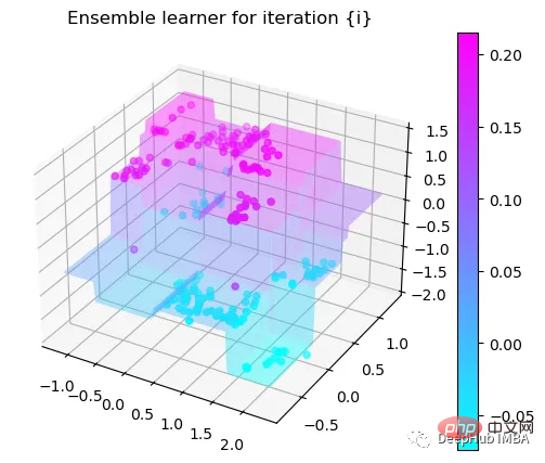
第6次决策

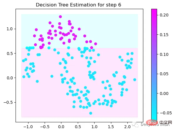
Tree Split for 1 and level 0.022058885544538498

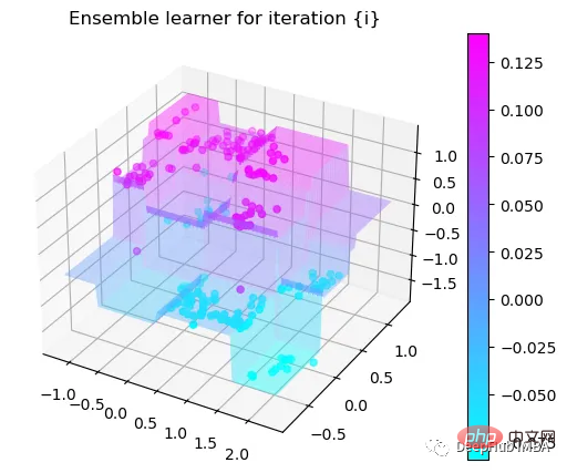
第7次决策

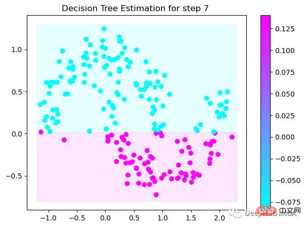
Tree Split for 0 and level -0.3030575215816498

第8次决策

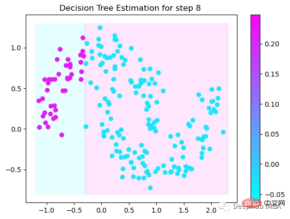
Tree Split for 0 and level 0.6119407713413239

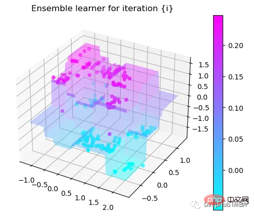
第9次决策

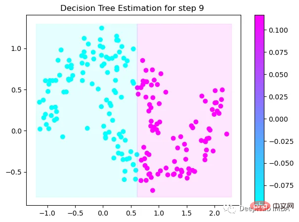
可以看到通过9次的计算，基本上已经把上面的分类进行了区分

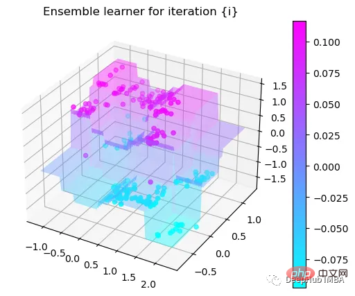
我们这里的学习器都是非常简单的决策树，只沿着一个特征分裂!但整体模型在每次决策后边的越来越复杂，并且整体误差逐渐减小。

plt.plot(rmses)

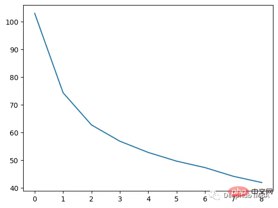
这也就是上图中我们看到的能够正确区分出了大部分的分类

如果你感兴趣可以使用下面代码自行实验：

​​//m.sbmmt.com/link/bfc89c3ee67d881255f8b097c4ed2d67​​

The above is the detailed content of Step-by-step visualization of the decision-making process of the gradient boosting algorithm. For more information, please follow other related articles on the PHP Chinese website!