This article brings you relevant knowledge about excel, which mainly introduces the related issues about multi-interval judgment. Everyone must have encountered the problem of multi-interval judgment, such as performance evaluation. , performance appraisal, etc. Let’s take a look at how to implement it. I hope it will be helpful to everyone.

Related learning recommendations: excel tutorial
Everyone must have encountered the problem of multi-interval judgment, such as score evaluation and performance Assessment and so on. Today I will share with you a function formula routine for multi-interval judgment.
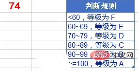
Let’s look at the problem first. The corresponding grade must be given based on the performance in cell A1. The division rule is:
60~69, the grade is "E";
70~79, the grade is "D";
80~89, the grade is "C";
90 ~99, the grade is "B";
>=100, the grade is "A".

Let’s briefly summarize the commonly used solutions and ideas.
=IF(A1>=100,"A",IF(A1>=90,"B",IF(A1>=80,"C", IF(A1>=70,"D",IF(A1>=60,"E","F")))))
Judge A1 layer by layer like peeling an onion through nesting of IF functions The interval within which the value lies, and the corresponding result is returned.
If it is greater than or equal to 100, return "A"; if it is greater than or equal to 90, return "B"; if it is greater than or equal to 80, return "C"...
The advantage of this formula is that it is easy to understand, but the disadvantage is If there are multiple judgment conditions, the formula will become longer and longer.
There is another question. When using the IF function to judge multiple intervals, friends can remember a trick, that is, you can start from the highest rule part and judge downward step by step. You can also start from the lowest rule section and work your way up. The formula just now can be written as:
=IF(A1
=LOOKUP(A1,{0,60 ,70,80,90,100},{"F","E","D","C","B","A"})
This way of writing is multi-interval judgment And returns the patterned formula of the corresponding value, which is an upgraded version of the layer-by-layer judgment of the IF function.
Note that the second parameter of LOOKUP must be processed in ascending order {0,60,70,80,90,100}.
The LOOKUP function uses A1 as the search value and returns the maximum value in the second parameter that is less than or equal to A1, that is, to find the eldest brother among all the younger brothers, and the third parameter {"F", "E", The string corresponding to the position in "D", "C", "B", "A"}.
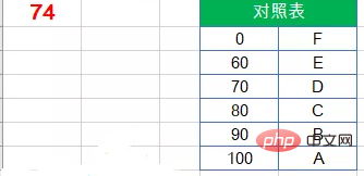
The next method does not seem awesome enough. You need to create a comparison table in Excel first:

Then use the VLOOKUP function to perform an approximate matching query in the comparison table:
=VLOOKUP(A1,D2:E7,2)
There are two points here Note:
1. The first column in the comparison table is sorted in ascending order;
2. The VLOOKUP function omits the fourth parameter and returns an exact matching value or an approximate matching value. If an exact matching value is not found, the maximum value smaller than the content to be queried (A1) is returned.
Compared with other formulas, the method of establishing a comparison table seems cumbersome, but in practical applications it is more convenient to modify the standards without having to re-edit the formula.
=MID("FEDCBA",MATCH(A1,{0,60,70,80,90,100}),1)
The function of the MATCH function is to query the position of a certain content in a row or column.
In this example, the MATCH function uses the content of cell A1 as the query value, uses approximate matching to find the location of A1 in the second parameter {0,60,70,80,90,100}, and returns The result is used as the second parameter of the MID function.
The MID function intercepts the string in the text string "FEDCBA". The specified starting position of the interception is the result calculated by the MATCH function. The length of the intercepted string is 1.
This formula is relatively complicated. Friends who don’t understand it don’t have to worry about it. Just understand it briefly.
Related learning recommendations: excel tutorial
The above is the detailed content of Detailed explanation of Excel examples to achieve multi-interval judgment. For more information, please follow other related articles on the PHP Chinese website!
 Compare the similarities and differences between two columns of data in excel
 excel duplicate item filter color
 How to copy an Excel table to make it the same size as the original
 Excel table slash divided into two
 Excel diagonal header is divided into two
 Absolute reference input method
 java export excel
 Excel input value is illegal


