This article brings you relevant knowledge aboutexcel, which mainly introduces the relevant content about the AGGREGATE function. The usage of this function is similar to the SUBTOTAL function, but it is more functional than the SUBTOTAL function. It's powerful, let's take a look at it, I hope it will be helpful to everyone.
Related learning recommendations:excel tutorial
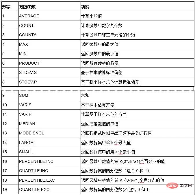
The usage of the AGGREGATE function is similar to the SUBTOTAL function, but it is more powerful than the SUBTOTAL function. , not only can realize the functions of 19 functions such as SUM, AVERAGE, COUNT, LARGE, MAX, etc., but also can ignore hidden rows, error values, null values, etc., and supports constant arrays.
The first parameter of this function is a number between 1 and 19, used to specify the summary method to be used:
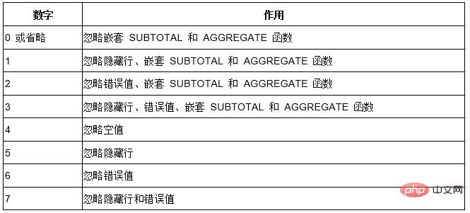
The second parameter is the A number between 0 and 7, specifying which types of values to ignore in the calculation area:
Next let’s talk about some typical uses of this function:
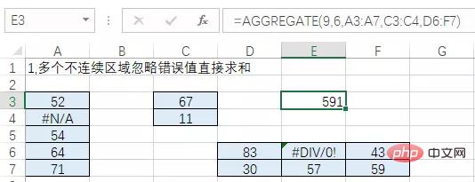
The power of this function is that the 2nd parameter can be specified to ignore error values and directly count
As follows Figure, the blue area contains different error values, now we need to sum these discontinuous areas.
The formula is:
=AGGREGATE(9,6,A3:A7,C3:C4,D6:F7)
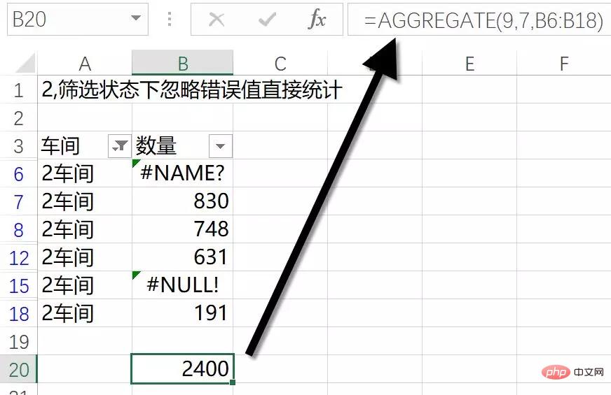
As shown below, the filtered data area contains error values. How to count the visible cells?
The formula is:
=AGGREGATE(9,7,B6:B18)
=AGGREGATE({4;5;1;9;3;12},{5,0},B4:B14)
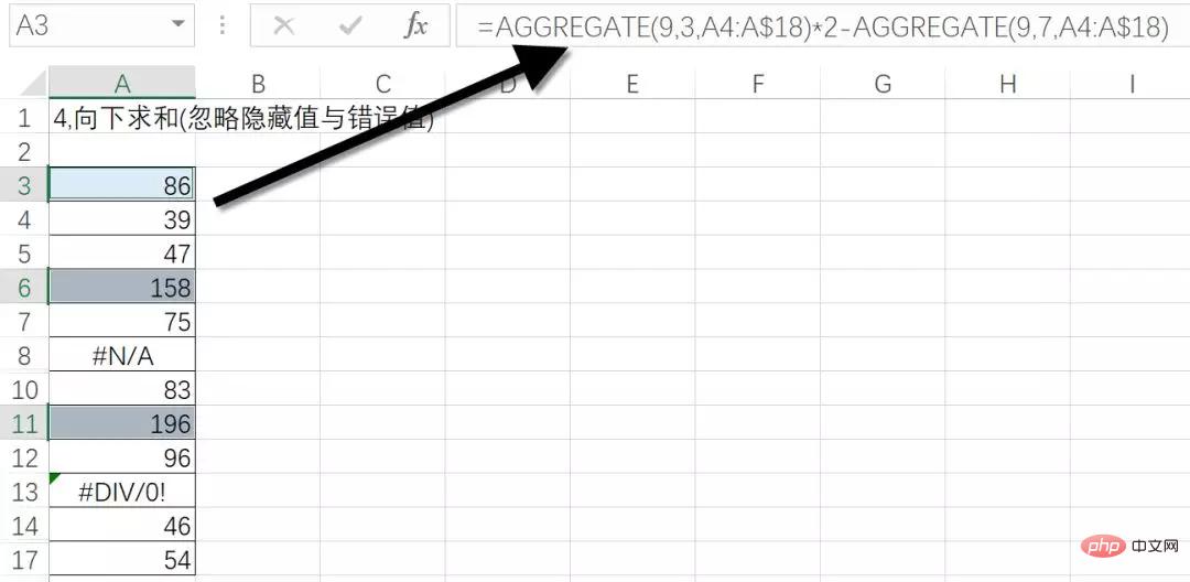
=AGGREGATE(9,3,A4:A$18)*2-AGGREGATE(9,7,A4:A$18)
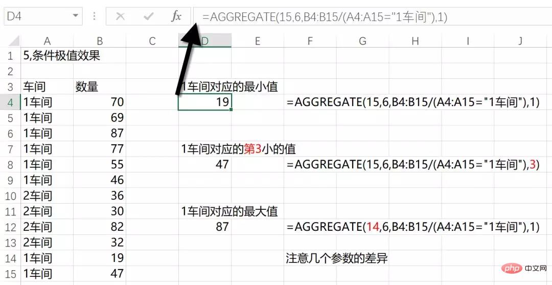
=AGGREGATE(15,6,B4:B15/(A4:A15="1 workshop" ),1)
=IFERROR(INDEX(B:B,AGGREGATE(15,6,ROW( $3:$12)/(A$3:A$12=D$3),ROW(A1))),"")
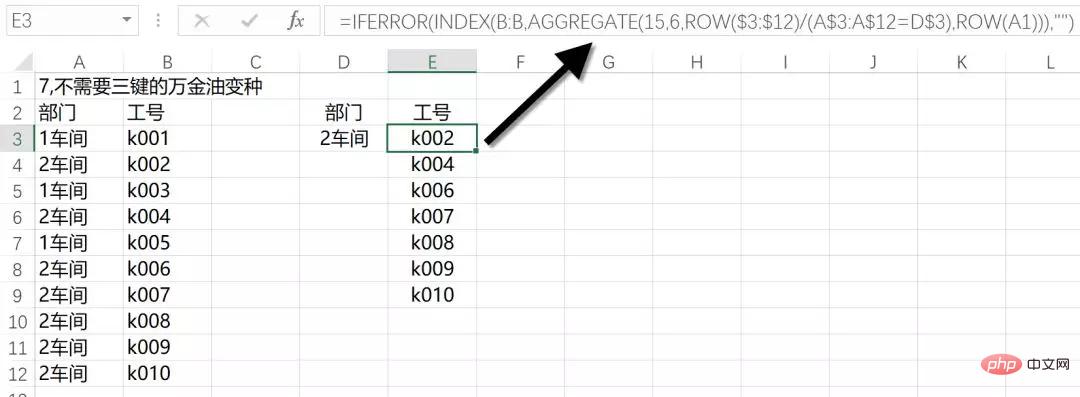
The idea of this formula is basically the same as the fifth formula.
As shown below, the assessment status of multiple people in column B is written in the same cell, and the maximum value must be counted. The formula is:
=AGGREGATE(14,6,--MID(B4,ROW($1:$50),COLUMN(A:AZ)),1)

For the MID(B4,ROW($1:$50),COLUMN(A:AZ)) part of the formula, use the MID function, starting from the 1st to 50th characters, and extract each A string with a length of 1~50 will result in a huge memory array. Use two more negative signs to turn the text in the memory array into an error value, and the value is still its own value.
Finally use the AGGREGATE function to ignore the error values in the memory array and calculate the first minimum value among them.
As shown in the figure below, it is necessary to count the maximum and minimum values corresponding to 1 workshop at the same time.
First select cells F4:G4 at the same time, enter the following formula in the edit bar, press Ctrl Shift and press Enter.
=AGGREGATE({16,15},6,B4:B15/(A4:A15=E4),1)
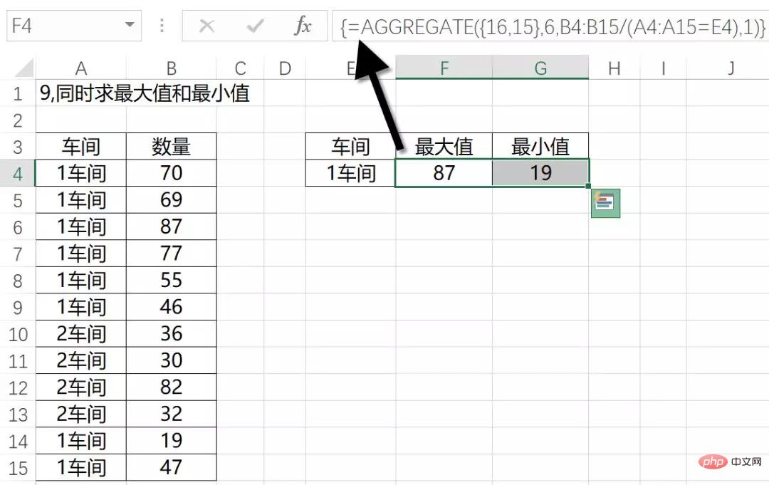
AGGREGATE The first parameter uses the constant array {16,15}, which indicates the calculation rules of using the maximum value and the minimum value respectively.
The final result is also a memory array, so two cells must be selected for input at the same time.
The characteristic of this function is that when the first parameter is 14~19, you can use the fourth parameter. At this time, the fourth parameter supports arrays, so you can play various applications to replace the direct SMALL, LARGE and other functions that ignore error values.
Related learning recommendations:excel tutorial
The above is the detailed content of Example summary of eight uses of the AGGREGATE function in Excel. For more information, please follow other related articles on the PHP Chinese website!
 Compare the similarities and differences between two columns of data in excel
 excel duplicate item filter color
 How to copy an Excel table to make it the same size as the original
 Excel table slash divided into two
 Excel diagonal header is divided into two
 Absolute reference input method
 java export excel
 Excel input value is illegal


