Let's talk about the simple and efficient Excel pivot table-excel-php.cn

This article brings you relevant knowledge aboutexcel, which mainly introduces simple and efficient Excel pivot table related operations, including creating a pivot table with dynamic data range, Let's take a look at the conversion of a two-dimensional table into a one-dimensional table and so on. I hope it will be helpful to everyone.

Let's talk about the simple and efficient Excel pivot table

Related learning recommendations:excel tutorial

The pivot table is simple to operate and easy to summarize. You can complete it with just a few clicks of the mouse. To analyze and summarize the data, today I will share a set of tips for using pivot tables.

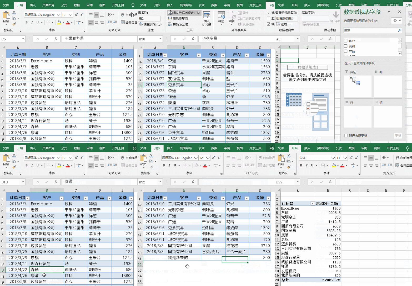
Create a pivot table with dynamic data range

The pivot table generated by default cannot be added to the pivot table after the data source adds data. In fact, before we make the pivot table, we insert the table first, and it's OK.

Use the automatic expansion feature of the table to provide a dynamic data source for the pivot table.

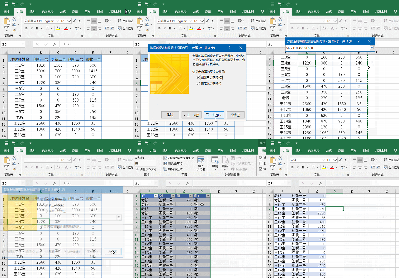
Lets talk about the simple and efficient Excel pivot table

Convert a two-dimensional table to a one-dimensional table

The so-called two-dimensional table usually refers to the same type of data appearing in multiple columns. Such a table does not To facilitate our summary analysis. How to convert it into a one-dimensional table in the form of a running account?

Press the Alt D P keys in sequence, select the multiple consolidated calculation data area, insert the default pivot table, and double-click "Total" in the lower right corner to get detailed data.

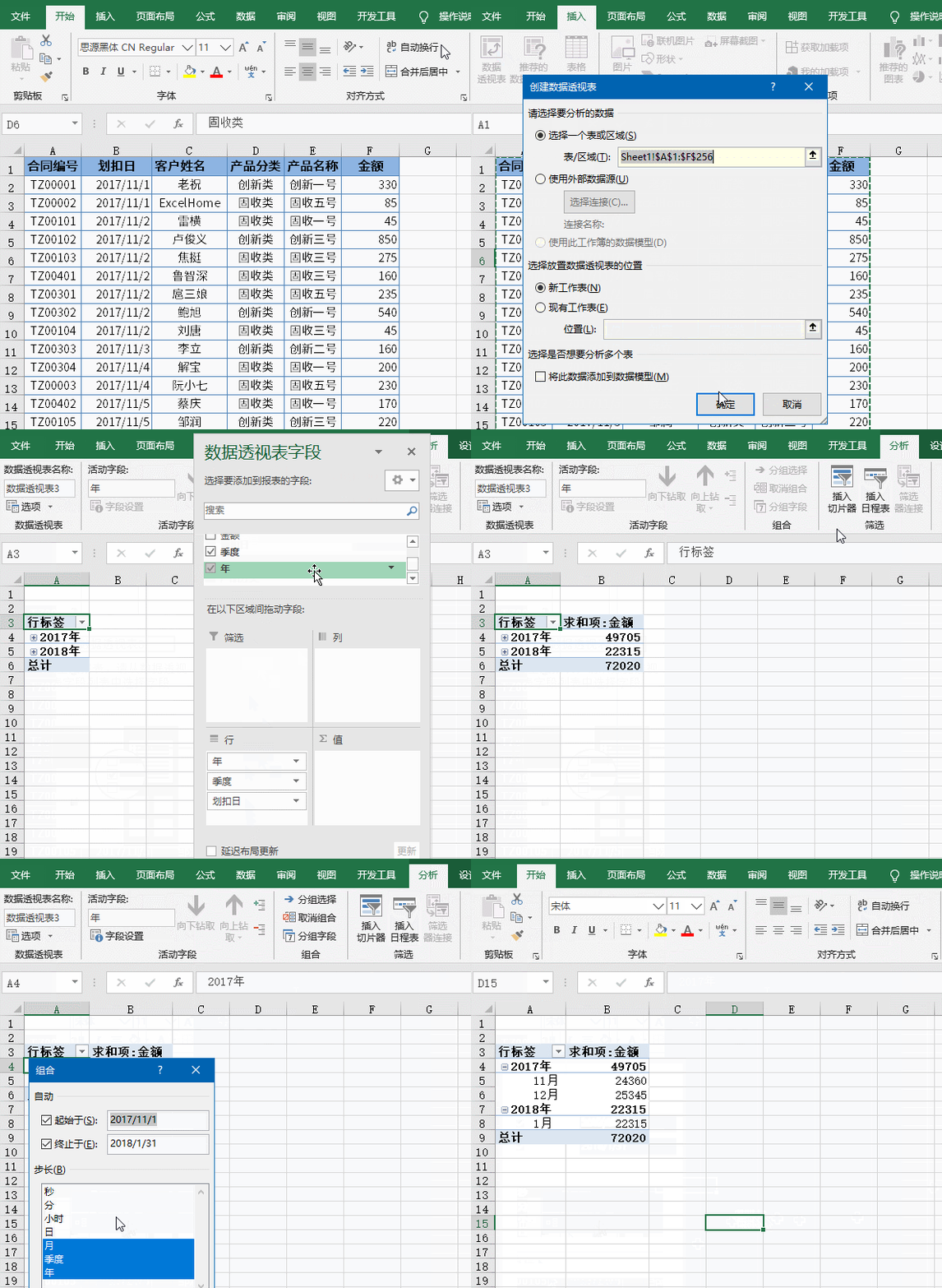
Lets talk about the simple and efficient Excel pivot table

Quickly summarize sales data by year, month, and quarter

Use the combination function in the pivot table to quickly summarize data by year, month, and quarter.

Lets talk about the simple and efficient Excel pivot table

Sales performance ranking and summary

To get the sales summary, sales ranking and sales proportion of different salesmen, as long as we choose different value summary methods Just OK.

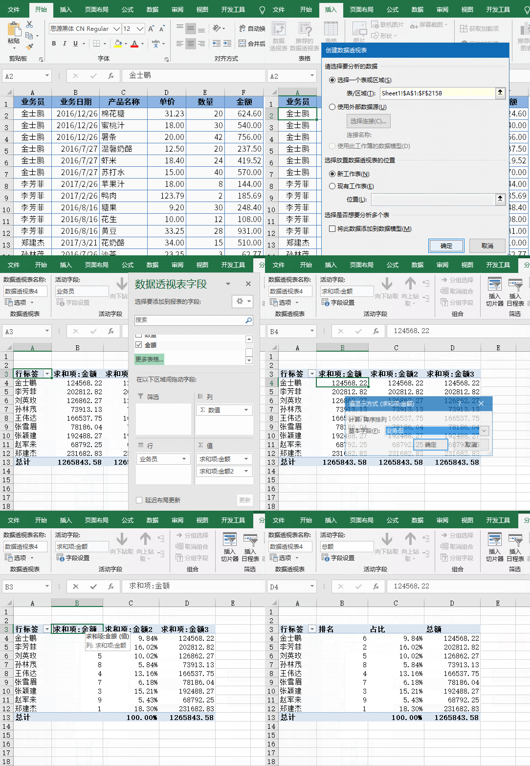
Lets talk about the simple and efficient Excel pivot table

Extract the top three sales records by sales area

Some seemingly complex summary requirements are very simple to complete using a pivot table.

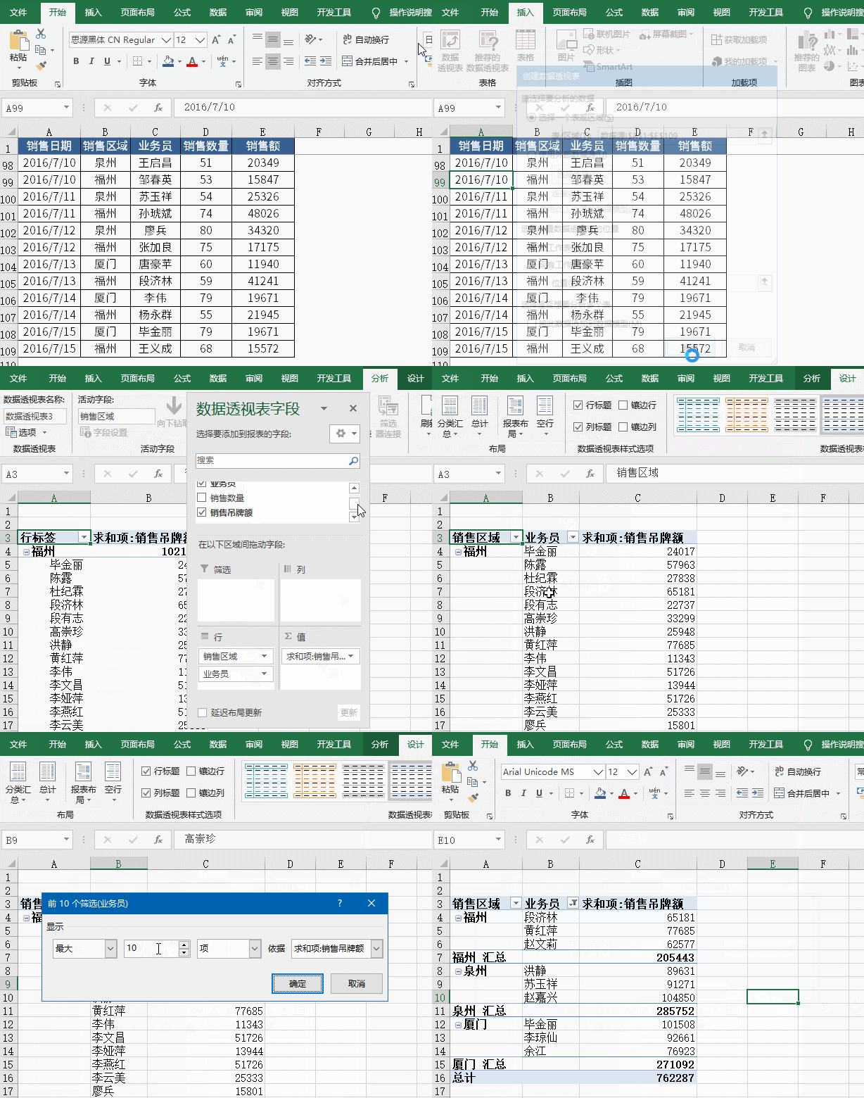
If you want to extract the top three sales records according to different sales areas, just do a filter in the pivot table.

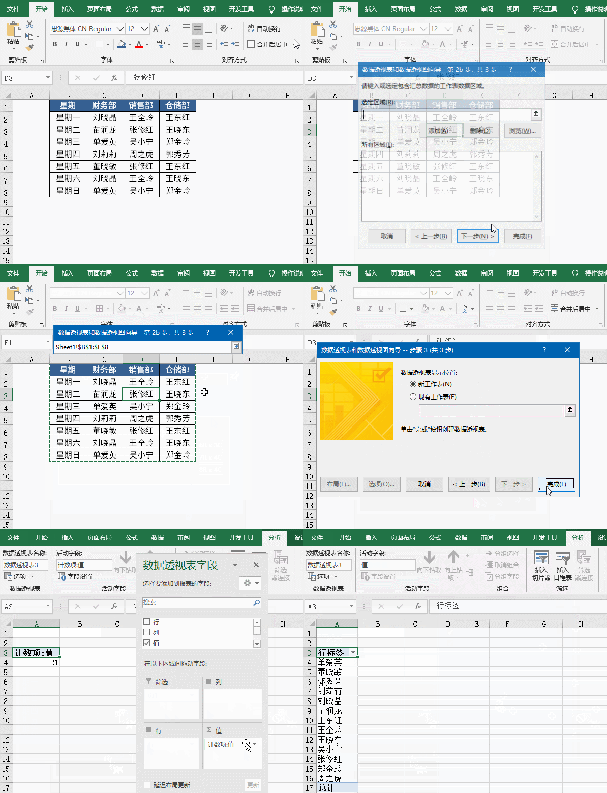
Lets talk about the simple and efficient Excel pivot table

Extract unique names from multiple rows and multiple columns

How to extract unique names from a duty list with multiple rows and multiple columns?

Press the Alt D P keys in sequence, select the multiple combined calculation data area, and insert the default pivot table.

In the PivotTable field list, drag "Page 1", "Row" and "Column" out of the field list respectively, and then drag "Value" to the row area.

Since when using multiple combined calculation areas, the first column in the data source will be used as the row label by default, so when selecting the data area, the first column cannot contain the name to be extracted.

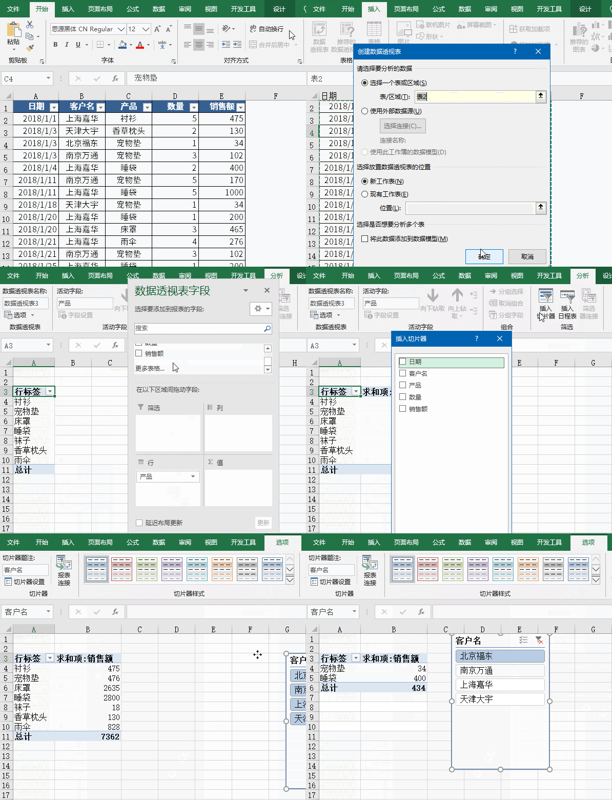
Lets talk about the simple and efficient Excel pivot table

Use the slicer to view sales data in different regions

The slicer is like an advanced filter that can make the filtering process more intuitive. In 2010 and above It would be a shame not to use a slicer in this version.

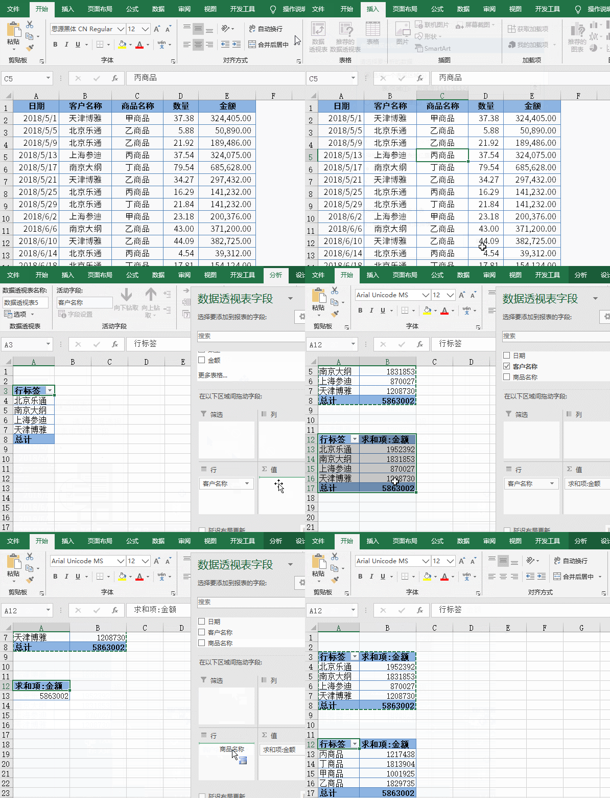
Lets talk about the simple and efficient Excel pivot table

Clone PivotTable

Select a PivotTable and press Ctrl C to copy, then press Ctrl V to paste, you can quickly get a new PivotTable , as long as you adjust the field position, you can get two pivot tables with different summary angles.

Lets talk about the simple and efficient Excel pivot table

Use slicers to control multiple pivot tables

For pivot tables generated using the same data source, you can first insert a slicer and then set the slicer The report connection enables it to control multiple pivot tables at the same time to achieve linkage effects.

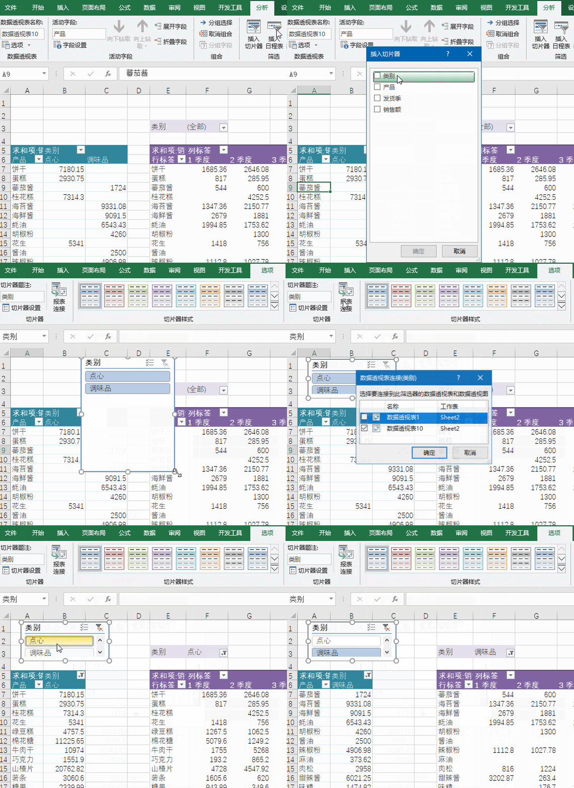
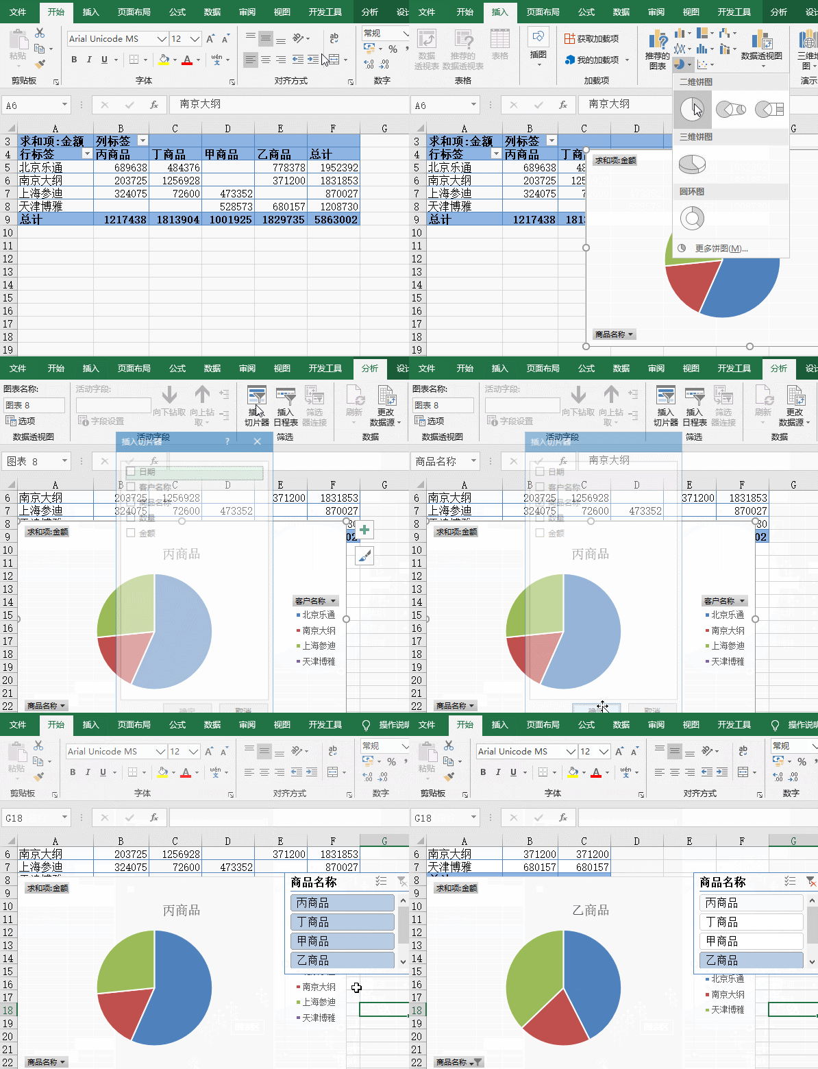
Lets talk about the simple and efficient Excel pivot table

Use slicers to create dynamic charts

The legendary interactive chart is quite simple to use a pivot chart.

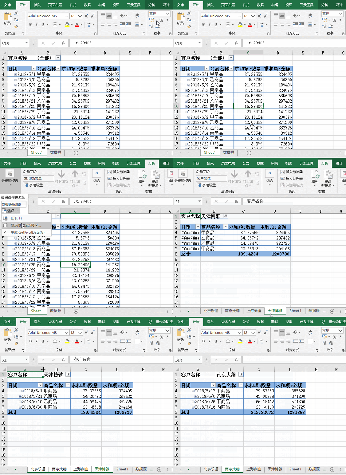
Lets talk about the simple and efficient Excel pivot table

Split the worksheet by customer

It is simple and unnecessary to split the data into different worksheet according to different customer names.

1111Lets talk about the simple and efficient Excel pivot table

Related learning recommendations:excel tutorial

The above is the detailed content of Let's talk about the simple and efficient Excel pivot table. For more information, please follow other related articles on the PHP Chinese website!