How to freeze selected area in excel

#How to freeze the selected area in Excel?

The steps to freeze the selected area in the EXCEL worksheet are as follows:

Required materials: computer, EXCEL

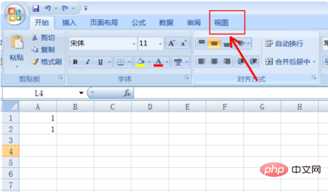
1. Open the target document and click on the top of the screen Select [View]

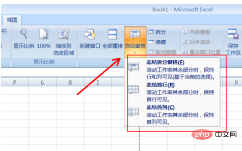
# on the toolbar. 2. If you want to freeze the first row or column, click the inverted triangle below to select the corresponding option.

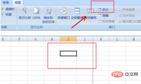
3. If you want to freeze other rows or columns, you must split them first: select a cell, and then click [View]-[Split]

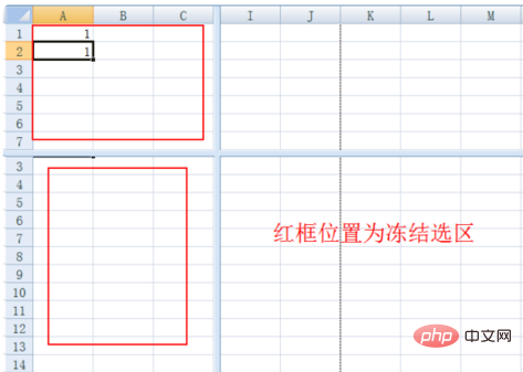
4. Then select [Freeze Panes]. After splitting, you can see a cross cursor. The columns to the left of the cursor and the rows above it are frozen for selection.

For more Excel-related technical articles, please visit theExcel Basic Tutorialcolumn!

The above is the detailed content of How to freeze selected area in excel. For more information, please follow other related articles on the PHP Chinese website!