Detailed introduction to how to use Naive Bayes algorithm in python

This article mainly introduces the relevant knowledge of how to use the Naive Bayes algorithm in Python. Has very good reference value. Let’s take a look at it with the editor

Here I’ll repeat why the title is “use” instead of “implementation”:

First of all, the algorithms provided by professionals are better than the algorithms we write ourselves. Both efficiency and accuracy are high.

Secondly, for people who are not good at mathematics, it is very painful to study a bunch of formulas in order to implement the algorithm.

Again, unless the algorithms provided by others cannot meet your needs, there is no need to "reinvent the wheel".

Let’s get back to the point. If you don’t know the Bayesian algorithm, you can check the relevant information. Here is just a brief introduction:

1. Bayesian formula:

P(A|B)=P(AB)/P(B)

2. Bayesian inference:

P(A|B)=P(A)×P(B|A)/P(B)

Express in words:

Posterior probability = prior probability × similarity/standardized constant

The problem that the Bayesian algorithm needs to solve is how to find the similarity, that is: P(B|A ) value

3. Three commonly used naive Bayes algorithms are provided in the scikit-learn package, which are explained in turn below:

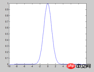
1) Gaussian Naive Bayes: Assume that attributes/features obey the normal distribution (as shown below), and is mainly used for numerical features.

Use the data that comes with the scikit-learn package. The code and description are as follows:

>>>from sklearn import datasets ##导入包中的数据
>>> iris=datasets.load_iris() ##加载数据
>>> iris.feature_names  ##显示特征名字
 ['sepal length (cm)', 'sepal width (cm)', 'petal length (cm)', 'petal width (cm)']
>>> iris.data   ##显示数据
 array([[ 5.1, 3.5, 1.4, 0.2],[ 4.9, 3. , 1.4, 0.2],[ 4.7, 3.2, 1.3, 0.2]............
>>> iris.data.size  ##数据大小 ---600个
>>> iris.target_names  ##显示分类的名字 
 array([&#39;setosa&#39;, &#39;versicolor&#39;, &#39;virginica&#39;], dtype=&#39;<U10&#39;)
>>> from sklearn.naive_bayes import GaussianNB ##导入高斯朴素贝叶斯算法
>>> clf = GaussianNB()    ##给算法赋一个变量，主要是为了方便使用
>>> clf.fit(iris.data, iris.target)  ##开始分类。对于量特别大的样本，可以使用函数partial_fit分类，避免一次加载过多数据到内存

>>> clf.predict(iris.data[0].reshape(1,-1)) ##验证分类。标红部分特别说明：因为predict的参数是数组，data[0]是列表，所以需要转换一下
array([0])
>>> data=np.array([6,4,6,2])   ##验证分类
>>> clf.predict(data.reshape(1,-1))
array([2])

There is a problem involved here: How to judge whether the data conforms to the normal distribution? There are related function judgments in the R language, or you can see it through direct drawing, but it is all a situation where P(x,y) can be drawn directly in the coordinate system. What about the data in the example? OK, I haven’t figured it out yet, this part will be added later.

2) Multinomial distribution Naive Bayes: often used for text classification, the feature is the word, and the value is the number of times the word appears.

##示例来在官方文档，详细说明见第一个例子
>>> import numpy as np
>>> X = np.random.randint(5, size=(6, 100)) ##返回随机整数值：范围[0,5) 大小6*100 6行100列
>>> y = np.array([1, 2, 3, 4, 5, 6])
>>> from sklearn.naive_bayes import MultinomialNB
>>> clf = MultinomialNB()
>>> clf.fit(X, y)
MultinomialNB(alpha=1.0, class_prior=None, fit_prior=True) 
>>> print(clf.predict(X[2]))
[3]

3) Bernoulli Naive Bayes: Each feature is of Boolean type, and the result is 0 or 1, that is, it does not appear.

##示例来在官方文档，详细说明见第一个例子
>>> import numpy as np
>>> X = np.random.randint(2, size=(6, 100))
>>> Y = np.array([1, 2, 3, 4, 4, 5])
>>> from sklearn.naive_bayes import BernoulliNB
>>> clf = BernoulliNB()
>>> clf.fit(X, Y)
BernoulliNB(alpha=1.0, binarize=0.0, class_prior=None, fit_prior=True) 
>>> print(clf.predict(X[2]))
[3]

The above is the detailed content of Detailed introduction to how to use Naive Bayes algorithm in python. For more information, please follow other related articles on the PHP Chinese website!