Detailed explanation of commonly used search data structures and algorithms (Python implementation)

1. Basic concepts

Searching is to determine a data element (or record) whose key is equal to the given value in the lookup table based on a given value.

Search Table: A collection of data elements (or records) of the same type

Keyword: the value of a data item in the data element , also called key value.

Primary Key: A keyword that uniquely identifies a data element or record.

Lookup tables can be divided into:

Static Search Table: A lookup table that only performs search operations. Its main operation is:

Query whether a "specific" data element is in the table

Retrieve a "specific" data element and various attributes

Dynamic Search Table: perform operations such as inserting or deleting at the same time during search:

Insert data during search

Delete data during search

2. Unordered Table lookup

is a linear search that traverses data elements without sorting the data.

Algorithm analysis: The best case is that it is found at the first position, which is O(1); the worst case is that it is found at the last position, which is O(n); so The average number of searches is (n+1)/2. The final time complexity is O(n)

# 最基础的遍历无序列表的查找算法
# 时间复杂度O(n)
 
def sequential_search(lis, key):
  length = len(lis)
  for i in range(length):
    if lis[i] == key:
      return i
    else:
      return False
 
 
if __name__ == '__main__':
  LIST = [1, 5, 8, 123, 22, 54, 7, 99, 300, 222]
  result = sequential_search(LIST, 123)
  print(result)

3. Ordered table lookup

The data in the lookup table must be sorted according to a primary key!

1. Binary Search

The core of the algorithm: Continuously compare the middle elements in the lookup table with the lookup value, and reduce the table range at a factor of half.

# 针对有序查找表的二分查找算法
# 时间复杂度O(log(n))
 
def binary_search(lis, key):
  low = 0
  high = len(lis) - 1
  time = 0
  while low < high:
    time += 1
    mid = int((low + high) / 2)
    if key < lis[mid]:
      high = mid - 1
    elif key > lis[mid]:
      low = mid + 1
    else:
      # 打印折半的次数
      print("times: %s" % time)
      return mid
  print("times: %s" % time)
  return False
 
if __name__ == &#39;__main__&#39;:
  LIST = [1, 5, 7, 8, 22, 54, 99, 123, 200, 222, 444]
  result = binary_search(LIST, 99)
  print(result)

2. Interpolation search

Although the binary search method is already very good, there are still areas that can be optimized.

Sometimes, filtering in half is not harsh enough. Wouldn’t it be better if nine-tenths of the data were excluded every time? Choosing this value is the key issue. The meaning of interpolation is: to reduce at a faster speed.

The core of interpolation is to use the formula:

value = (key - list[low])/(list[high] - list[low])

Use this value to replace 1/2 in binary search.

The above code can be used directly, you only need to change one sentence.

# 插值查找算法
# 时间复杂度O(log(n))
 
def binary_search(lis, key):
  low = 0
  high = len(lis) - 1
  time = 0
  while low < high:
    time += 1
    # 计算mid值是插值算法的核心代码
    mid = low + int((high - low) * (key - lis[low])/(lis[high] - lis[low]))
    print("mid=%s, low=%s, high=%s" % (mid, low, high))
    if key < lis[mid]:
      high = mid - 1
    elif key > lis[mid]:
      low = mid + 1
    else:
      # 打印查找的次数
      print("times: %s" % time)
      return mid
  print("times: %s" % time)
  return False
 
if __name__ == &#39;__main__&#39;:
  LIST = [1, 5, 7, 8, 22, 54, 99, 123, 200, 222, 444]
  result = binary_search(LIST, 444)
  print(result)

The overall time complexity of the interpolation algorithm is still at the O(log(n)) level. The advantage is that for lookup tables with a large amount of data in the table and relatively even distribution of keywords, the average performance of using the interpolation algorithm is much better than binary search. On the contrary, for data with extremely uneven distribution, the interpolation algorithm is not suitable.

3. Fibonacci search

Inspired by the interpolation algorithm, the Fibonacci algorithm was invented. The core is also how to optimize the reduction rate so that the number of searches is minimized.

To use this algorithm, the premise is that there is already a list containing Fibonacci data

F = [1, 1, 2, 3, 5, 8 , 13, 21, 34, 55, 89, 144,...]

# 斐波那契查找算法
# 时间复杂度O(log(n))
 
def fibonacci_search(lis, key):
  # 需要一个现成的斐波那契列表。其最大元素的值必须超过查找表中元素个数的数值。
  F = [1, 1, 2, 3, 5, 8, 13, 21, 34, 55, 89, 144,
     233, 377, 610, 987, 1597, 2584, 4181, 6765,
     10946, 17711, 28657, 46368]
  low = 0
  high = len(lis) - 1
   
  # 为了使得查找表满足斐波那契特性，在表的最后添加几个同样的值
  # 这个值是原查找表的最后那个元素的值
  # 添加的个数由F[k]-1-high决定
  k = 0
  while high > F[k]-1:
    k += 1
  print(k)
  i = high
  while F[k]-1 > i:
    lis.append(lis[high])
    i += 1
  print(lis)
   
  # 算法主逻辑。time用于展示循环的次数。
  time = 0
  while low <= high:
    time += 1
    # 为了防止F列表下标溢出，设置if和else
    if k < 2:
      mid = low
    else:
      mid = low + F[k-1]-1
     
    print("low=%s, mid=%s, high=%s" % (low, mid, high))
    if key < lis[mid]:
      high = mid - 1
      k -= 1
    elif key > lis[mid]:
      low = mid + 1
      k -= 2
    else:
      if mid <= high:
        # 打印查找的次数
        print("times: %s" % time)
        return mid
      else:
        print("times: %s" % time)
        return high
  print("times: %s" % time)
  return False
 
if __name__ == &#39;__main__&#39;:
  LIST = [1, 5, 7, 8, 22, 54, 99, 123, 200, 222, 444]
  result = fibonacci_search(LIST, 444)
  print(result)

Algorithm analysis: The overall time complexity of Fibonacci search is also O(log(n )). But in terms of average performance, it is better than binary search. But in the worst case, for example, if the key is 1 here, the search is always in the left half area. At this time, its efficiency is lower than binary search.

Summary: The mid operation of binary search is addition and division, the interpolation search is the complex four arithmetic operations, and the Fibonacci search is just the simplest addition and subtraction operation. In searching massive data, this subtle difference may affect the final search efficiency. Therefore, the three search methods for ordered tables are essentially different in the selection of split points. Each has its own advantages and disadvantages, and the choice should be based on the actual situation.

4. Linear index search

For massive unordered data, in order to improve the search speed, an index table is generally constructed for it.

Indexing is the process of associating a keyword with its corresponding record.

An index consists of several index items. Each index item contains at least information such as keywords and their corresponding record locations in the memory.

Indices can be divided into linear indexes, tree indexes and multi-level indexes according to their structures.

Linear index: Organize the collection of index items through a linear structure, also called an index table.

Linear index can be divided into: dense index, block index and inverted index

1.Dense index

Dense index refers to online In a sexual index, an index entry is created for each record in the data collection.

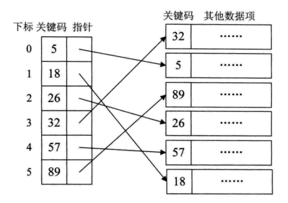
#This is actually equivalent to establishing an ordered linear list for an unordered set. The index items must be arranged in order according to the key code.

This is also equivalent to doing the sorting work required in the search process in advance.

1. Block index

Blocks a large number of unordered data sets, so that there is no order within the block and order between blocks.

这其实是有序查找和无序查找的一种中间状态或者说妥协状态。因为数据量过大，建立完整的稠密索引耗时耗力，占用资源过多；但如果不做任何排序或者索引，那么遍历的查找也无法接受，只能折中，做一定程度的排序或索引。

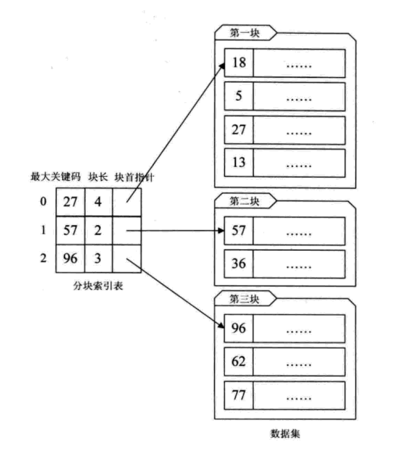
分块索引的效率比遍历查找的O(n)要高一些，但与二分查找的O(logn)还是要差不少。

1.倒排索引

不是由记录来确定属性值，而是由属性值来确定记录的位置，这种被称为倒排索引。其中记录号表存储具有相同次关键字的所有记录的地址或引用（可以是指向记录的指针或该记录的主关键字）。

倒排索引是最基础的搜索引擎索引技术。

五、二叉排序树

二叉排序树又称为二叉查找树。它或者是一颗空树，或者是具有下列性质的二叉树：

若它的左子树不为空，则左子树上所有节点的值均小于它的根结构的值；

若它的右子树不为空，则右子树上所有节点的值均大于它的根结构的值；

它的左、右子树也分别为二叉排序树。

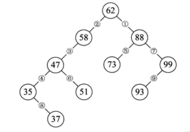
构造一颗二叉排序树的目的，往往不是为了排序，而是为了提高查找和插入删除关键字的速度。

二叉排序树的操作：

1.查找：对比节点的值和关键字，相等则表明找到了；小了则往节点的左子树去找，大了则往右子树去找，这么递归下去，最后返回布尔值或找到的节点。

2.插入：从根节点开始逐个与关键字进行对比，小了去左边，大了去右边，碰到子树为空的情况就将新的节点链接。

3.删除：如果要删除的节点是叶子，直接删；如果只有左子树或只有右子树，则删除节点后，将子树链接到父节点即可；如果同时有左右子树，则可以将二叉排序树进行中序遍历，取将要被删除的节点的前驱或者后继节点替代这个被删除的节点的位置。

#!/usr/bin/env python
# -*- coding:utf-8 -*-
# Author: Liu Jiang
# Python 3.5
 
 
class BSTNode:
  """
  定义一个二叉树节点类。
  以讨论算法为主，忽略了一些诸如对数据类型进行判断的问题。
  """
  def __init__(self, data, left=None, right=None):
    """
    初始化
    :param data: 节点储存的数据
    :param left: 节点左子树
    :param right: 节点右子树
    """
    self.data = data
    self.left = left
    self.right = right
 
 
class BinarySortTree:
  """
  基于BSTNode类的二叉排序树。维护一个根节点的指针。
  """
  def __init__(self):
    self._root = None
 
  def is_empty(self):
    return self._root is None
 
  def search(self, key):
    """
    关键码检索
    :param key: 关键码
    :return: 查询节点或None
    """
    bt = self._root
    while bt:
      entry = bt.data
      if key < entry:
        bt = bt.left
      elif key > entry:
        bt = bt.right
      else:
        return entry
    return None
 
  def insert(self, key):
    """
    插入操作
    :param key:关键码
    :return: 布尔值
    """
    bt = self._root
    if not bt:
      self._root = BSTNode(key)
      return
    while True:
      entry = bt.data
      if key < entry:
        if bt.left is None:
          bt.left = BSTNode(key)
          return
        bt = bt.left
      elif key > entry:
        if bt.right is None:
          bt.right = BSTNode(key)
          return
        bt = bt.right
      else:
        bt.data = key
        return
 
  def delete(self, key):
    """
    二叉排序树最复杂的方法
    :param key: 关键码
    :return: 布尔值
    """
    p, q = None, self._root   # 维持p为q的父节点，用于后面的链接操作
    if not q:
      print("空树！")
      return
    while q and q.data != key:
      p = q
      if key < q.data:
        q = q.left
      else:
        q = q.right
      if not q:        # 当树中没有关键码key时，结束退出。
        return
    # 上面已将找到了要删除的节点，用q引用。而p则是q的父节点或者None（q为根节点时）。
    if not q.left:
      if p is None:
        self._root = q.right
      elif q is p.left:
        p.left = q.right
      else:
        p.right = q.right
      return
    # 查找节点q的左子树的最右节点，将q的右子树链接为该节点的右子树
    # 该方法可能会增大树的深度，效率并不算高。可以设计其它的方法。
    r = q.left
    while r.right:
      r = r.right
    r.right = q.right
    if p is None:
      self._root = q.left
    elif p.left is q:
      p.left = q.left
    else:
      p.right = q.left
 
  def __iter__(self):
    """
    实现二叉树的中序遍历算法,
    展示我们创建的二叉排序树.
    直接使用python内置的列表作为一个栈。
    :return: data
    """
    stack = []
    node = self._root
    while node or stack:
      while node:
        stack.append(node)
        node = node.left
      node = stack.pop()
      yield node.data
      node = node.right
 
 
if __name__ == &#39;__main__&#39;:
  lis = [62, 58, 88, 48, 73, 99, 35, 51, 93, 29, 37, 49, 56, 36, 50]
  bs_tree = BinarySortTree()
  for i in range(len(lis)):
    bs_tree.insert(lis[i])
  # bs_tree.insert(100)
  bs_tree.delete(58)
  for i in bs_tree:
    print(i, end=" ")
  # print("\n", bs_tree.search(4))

二叉排序树总结：

二叉排序树以链式进行存储，保持了链接结构在插入和删除操作上的优点。

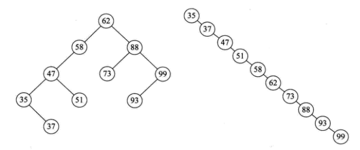
在极端情况下，查询次数为1，但最大操作次数不会超过树的深度。也就是说，二叉排序树的查找性能取决于二叉排序树的形状，也就引申出了后面的平衡二叉树。

给定一个元素集合，可以构造不同的二叉排序树，当它同时是一个完全二叉树的时候，查找的时间复杂度为O(log(n))，近似于二分查找。

当出现最极端的斜树时，其时间复杂度为O(n)，等同于顺序查找，效果最差。

六、 平衡二叉树

平衡二叉树（AVL树，发明者的姓名缩写）：一种高度平衡的排序二叉树，其每一个节点的左子树和右子树的高度差最多等于1。

平衡二叉树首先必须是一棵二叉排序树！

平衡因子（Balance Factor）：将二叉树上节点的左子树深度减去右子树深度的值。

对于平衡二叉树所有包括分支节点和叶节点的平衡因子只可能是-1,0和1，只要有一个节点的因子不在这三个值之内，该二叉树就是不平衡的。

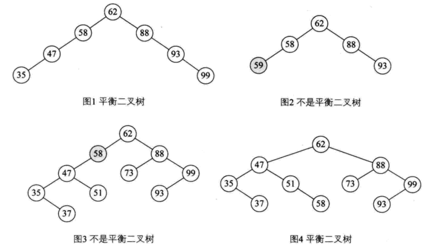
最小不平衡子树：距离插入结点最近的，且平衡因子的绝对值大于1的节点为根的子树。

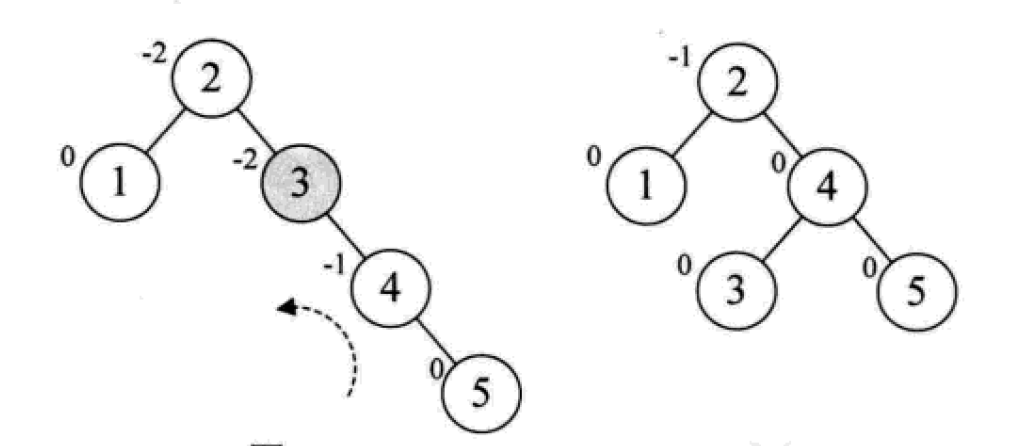
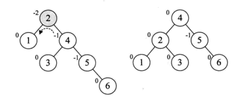
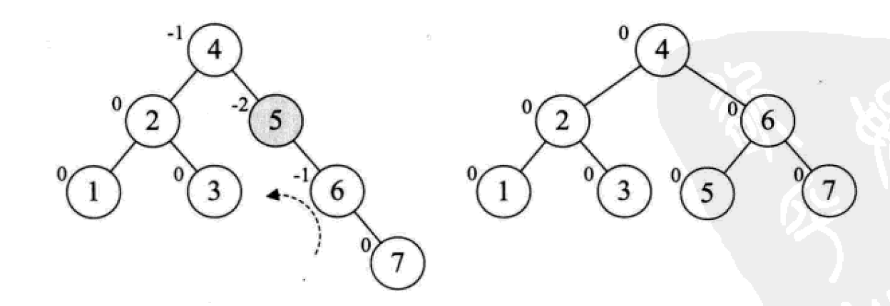
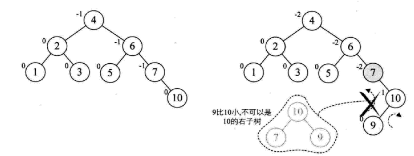
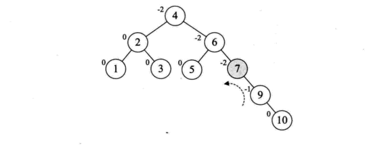
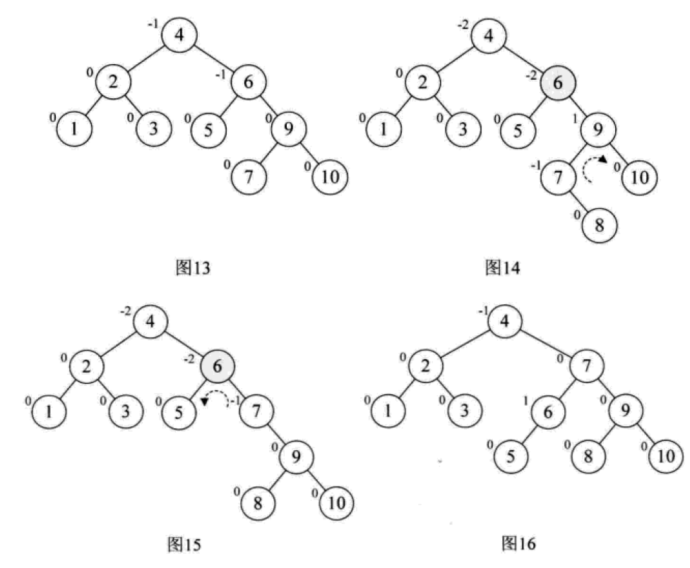
平衡二叉树的构建思想：每当插入一个新结点时，先检查是否破坏了树的平衡性，若有，找出最小不平衡子树。在保持二叉排序树特性的前提下，调整最小不平衡子树中各结点之间的连接关系，进行相应的旋转，成为新的平衡子树。

下面是由[1,2,3,4,5,6,7,10,9]构建平衡二叉树

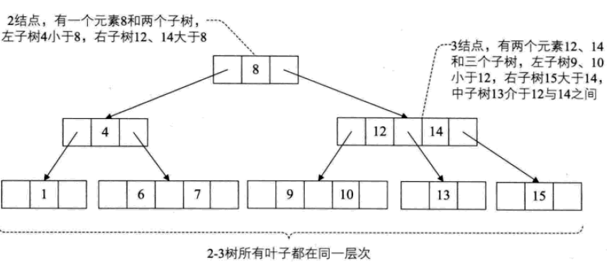
For multi-way search trees, the key is how many elements each node can store and the number of its children. There are four commonly used forms: 2-3 tree, 2-3-4 tree, and B tree. and B+ trees.

## The deletion operation is as follows:

2- 3-4 tree

is actually an extension of 2-3 tree, including the use of 4 nodes. A 4-node contains three elements, small, medium and large, and four children (or no children).

The insertion operation:

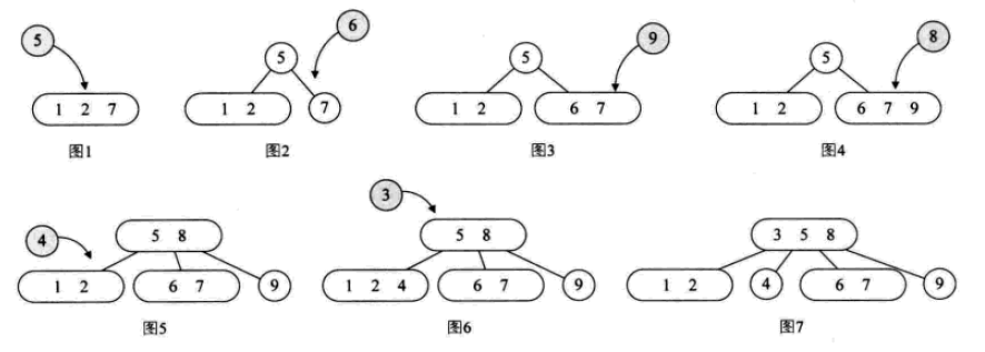
The deletion operation:

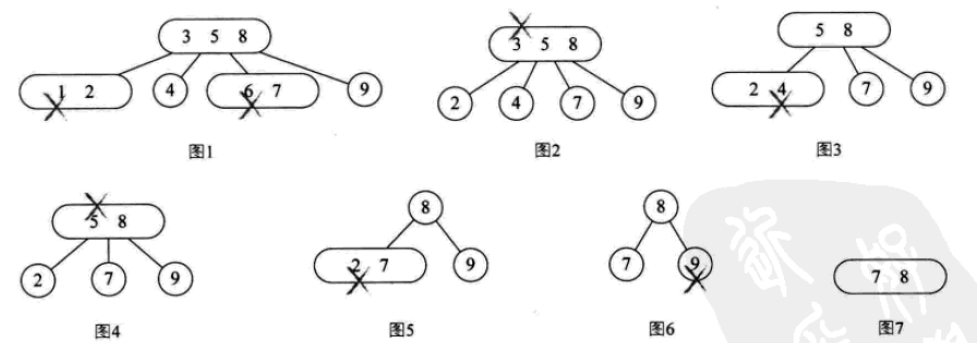
B tree

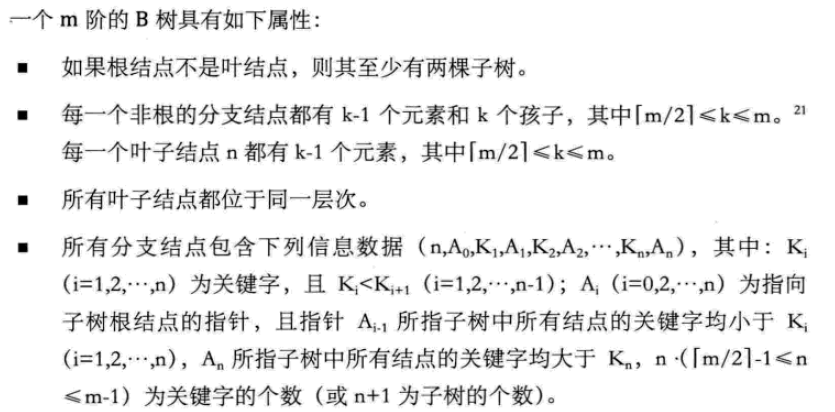
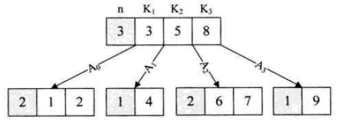
B tree is a balanced multi-way search tree. The maximum number of children of a node is called the order of the B-tree. The 2-3 tree is a third-order B-tree, and the 2-3-4 is a fourth-order B-tree.

The B-tree data structure is mainly used in data interaction between memory and external storage.

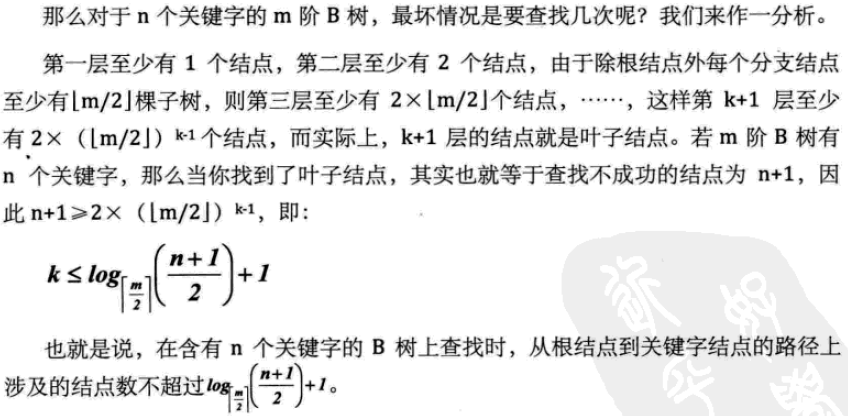
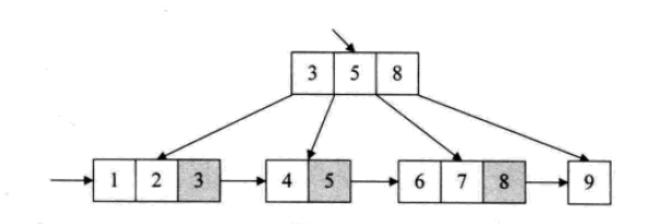
## The structure of the #B+ tree is particularly suitable for searches with ranges. For example, find people aged between 20 and 30 years old.

8. Hash table (hash table)

Hash table: There is no relationship between all elements. The storage location of the element is directly calculated through a function using the keyword of the element. This one-to-one relationship function is called a hash function or Hash function.

Use hashing technology to store records in a continuous storage space, called a hash table or hash table (Hash Table). The storage location corresponding to the keyword is called the hash address.

Hash table is a search-oriented storage structure. The problem it is best suited for is finding records equal to a given value. However, it is not suitable for situations where a certain keyword can correspond to many records, such as finding all "male" genders. It is also not suitable for range searches, such as searching for people between the ages of 20 and 30. Sorting, largest, smallest, etc. are also inappropriate.

Therefore, hash tables are usually used for data structures whose keywords are not repeated. For example, python's dictionary data type.

Designing a simple, uniform, and high storage utilization hash function is the most critical issue in hashing technology.

However, general hash functions face conflict problems.

Conflict: Two different keywords have the same result after being calculated by the hash function. collision.

8.1 Construction method of hash function

Good hash function: simple calculation, even distribution of hash addresses

1. Direct addressing method

For example, take a linear function of the keyword as a hash function:

f(key) = a*key + b (a, b are constants)

2.数字分析法

抽取关键字里的数字，根据数字的特点进行地址分配

3.平方取中法

将关键字的数字求平方，再截取部分

4.折叠法

将关键字的数字分割后分别计算，再合并计算，一种玩弄数字的手段。

5.除留余数法

最为常见的方法之一。

对于表长为m的数据集合，散列公式为：

f(key) = key mod p (p<=m)

mod：取模（求余数）

该方法最关键的是p的选择，而且数据量较大的时候，冲突是必然的。一般会选择接近m的质数。

6.随机数法

选择一个随机数，取关键字的随机函数值为它的散列地址。

f(key) = random(key)

总结，实际情况下根据不同的数据特性采用不同的散列方法，考虑下面一些主要问题：

计算散列地址所需的时间

关键字的长度

散列表的大小

关键字的分布情况

记录查找的频率

8.2 处理散列冲突

1、开放定址法

就是一旦发生冲突，就去寻找下一个空的散列地址，只要散列表足够大，空的散列地址总能找到，并将记录存入。

公式是：

这种简单的冲突解决办法被称为线性探测，无非就是自家的坑被占了，就逐个拜访后面的坑，有空的就进，也不管这个坑是不是后面有人预定了的。

线性探测带来的最大问题就是冲突的堆积，你把别人预定的坑占了，别人也就要像你一样去找坑。

改进的办法有二次方探测法和随机数探测法。

2、再散列函数法

发生冲突时就换一个散列函数计算，总会有一个可以把冲突解决掉，它能够使得关键字不产生聚集，但相应地增加了计算的时间。

3、链接地址法
碰到冲突时，不更换地址，而是将所有关键字为同义词的记录存储在一个链表里，在散列表中只存储同义词子表的头指针，如下图：

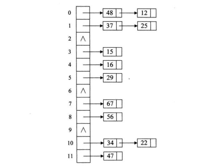
这样的好处是，不怕冲突多；缺点是降低了散列结构的随机存储性能。本质是用单链表结构辅助散列结构的不足。

4、公共溢出区法

其实就是为所有的冲突，额外开辟一块存储空间。如果相对基本表而言，冲突的数据很少的时候，使用这种方法比较合适。

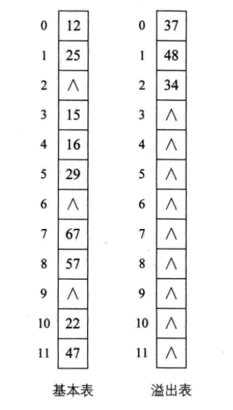
8.3 散列表查找实现

下面是一段简单的实现代码：

#!/usr/bin/env python
# -*- coding:utf-8 -*-
# Author: Liu Jiang
# Python 3.5
# 忽略了对数据类型，元素溢出等问题的判断。
 
 
class HashTable:
  def __init__(self, size):
    self.elem = [None for i in range(size)] # 使用list数据结构作为哈希表元素保存方法
    self.count = size # 最大表长
 
  def hash(self, key):
    return key % self.count # 散列函数采用除留余数法
 
  def insert_hash(self, key):
    """插入关键字到哈希表内"""
    address = self.hash(key) # 求散列地址
    while self.elem[address]: # 当前位置已经有数据了，发生冲突。
      address = (address+1) % self.count # 线性探测下一地址是否可用
    self.elem[address] = key # 没有冲突则直接保存。
 
  def search_hash(self, key):
    """查找关键字，返回布尔值"""
    star = address = self.hash(key)
    while self.elem[address] != key:
      address = (address + 1) % self.count
      if not self.elem[address] or address == star: # 说明没找到或者循环到了开始的位置
        return False
    return True
 
 
if __name__ == '__main__':
  list_a = [12, 67, 56, 16, 25, 37, 22, 29, 15, 47, 48, 34]
  hash_table = HashTable(12)
  for i in list_a:
    hash_table.insert_hash(i)
 
  for i in hash_table.elem:
    if i:
      print((i, hash_table.elem.index(i)), end=" ")
  print("\n")
 
  print(hash_table.search_hash(15))
  print(hash_table.search_hash(33))

8.4 散列表查找性能分析

如果没发生冲突，则其查找时间复杂度为O(1)，属于最极端的好了。

但是，现实中冲突可不可避免的，下面三个方面对查找性能影响较大：

散列函数是否均匀

处理冲突的办法

散列表的装填因子（表内数据装满的程度）

以上就是本文的全部内容，希望对大家的学习有所帮助，也希望大家多多支持PHP中文网。

更多Detailed explanation of commonly used search data structures and algorithms (Python implementation)相关文章请关注PHP中文网！