机器学习预测建模是指利用机器学习算法对现有数据进行分析和建模,从而预测未来的趋势和结果。这种方法已经被广泛应用于各个领域,如金融、医疗、交通和电子商务等。随着人们对数据的需求不断增加,同时计算机的处理能力和算法的发展也为机器学习预测建模提供了支持。在大数据时代,机器学习预测建模已经成为数据分析和决策制定的重要工具。
☞☞☞AI 智能聊天, 问答助手, AI 智能搜索, 免费无限量使用 DeepSeek R1 模型☜☜☜

机器学习预测建模是指利用机器学习算法对现有数据进行分析和建模,从而预测未来的趋势和结果。这种方法已经被广泛应用于各个领域,如金融、医疗、交通和电子商务等。随着人们对数据的需求不断增加,同时计算机的处理能力和算法的发展也为机器学习预测建模提供了支持。在大数据时代,机器学习预测建模已经成为数据分析和决策制定的重要工具。
在机器学习中,预测建模是十分关键的一步,特别是模型选择。模型选择在机器学习预测建模中具有非常重要的地位。模型选择的正确与否直接关系到预测的准确度和效果。在模型选择过程中,需要考虑多个因素,如模型的性能、泛化能力、计算成本、数据量等。在选择模型时,需要考虑模型的性能指标,如准确率、精度、召回率、F1分数等。准确率是评估模型预测能力的重要指标,精度则可以衡量模型预测结果与实际结果之间的差异程度,召回率和F1分数则可以综合考虑模型的预测精度和召回能力。
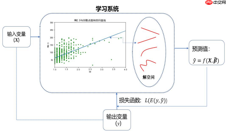
数据预测,简而言之就是基于已有数据集,归纳出输入变量和输出变量之间的数量关系。基于这种数量关系:
数据预测涉及的问题:
什么是预测模型?
立即学习“Python免费学习笔记(深入)”;
y=β0+β1X1+β2X2+...+βpXp+ε
log(1−PP)=β0+β1X1+β2X2+...+βpXp+ε
y^=β0^+β1^X1+β2^X2+...+βp^Xp
LogitP^=log(1−P^P^)=β0^+β1^X1+β2^X2+...+βp^Xp
预测模型的其他形式:
预测建模的出发点,是将数据集中的N个样本观测数据,视为p维实数空间Rp中的N个点
回归预测模型::
分类预测模型:
从直线到曲线,从平面到曲面 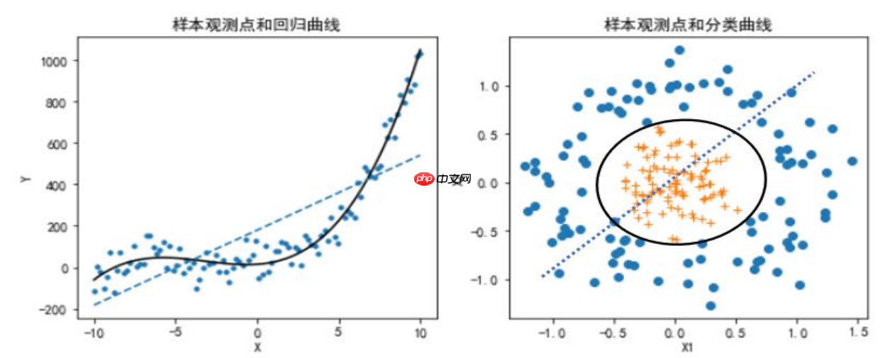
损失函数L是误差e的函数
L(e)=L(yi,yi^)=(yi−yi^)2
i=1∑NL(yi,yi^)=i=1∑N(yi−yi^)2
L(yi,pk^(Xi))=−k=1∑KI(yi=k)log(Pk^(Xi))=−logPyi^(Xi)
L(yi,f^(Xi))=−yif^(Xi)+log(1+exp(f^(Xi)))
L(yi,f^(Xi))=exp(−yif^(Xi))
L(yi,fk^(Xi))=−k=1∑KI(yi=k)log(suml=1Kexp(fl^(Xi))exp(fk^(Xi)))
i=1∑NL(yi,yi^)=i=1∑NL(yi,f^(Xi))=i=1∑N(yi−(β0^+β1^Xi1+β2^Xi2+...+βp^Xip))2
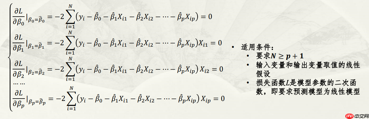
参数解空间和搜索策略:
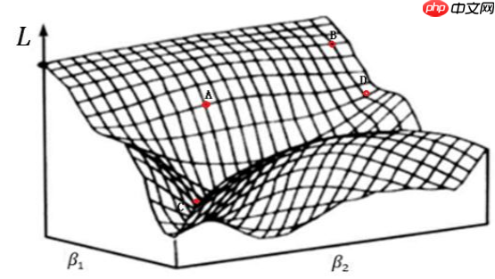
两个重要概念
讨论的问题:
(1)回归预测模型中的误差评价指标:均方误差(MSE)
MSE=N1i=1∑N(yi−yi^)2=E(L(yi,f^(Xi)))
(2)二分类预测模型中的误差评价指标
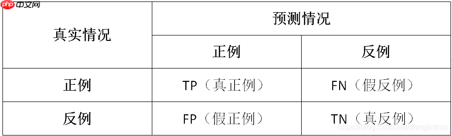
解释说明:
通俗理解 以西瓜数据集为例,我们来通俗理解一下什么是TP、TN、FP、FN。
(3)多分类预测模型中的误差评价指标:
# 代码实现ROC曲线和P-R曲线import pandas as pdimport numpy as npfrom matplotlib import pyplot as plt
%matplotlib inline#指定默认字体plt.rcParams['font.sans-serif']=['FZHuaLi-M14S']
plt.rcParams['axes.unicode_minus'] = Falsedata = pd.read_csv('类别和概率.csv')
label=data['label']
prob=data['prob']
pos = np.sum(label == 1)
neg = np.sum(label == 0)
prob_sort = np.sort(prob)[::-1]
index = np.argsort(prob)[::-1]
label_sort = label[index]

Pre = []
Rec = []
tpr=[]
fpr=[]for i, item in enumerate(prob_sort):
    Rec.append(np.sum((label_sort[:(i+1)] == 1)) /pos)
    Pre.append(np.sum((label_sort[:(i+1)] == 1))/(i+1))
    tpr.append(np.sum((label_sort[:(i+1)] == 1))/pos)
    fpr.append(np.sum((label_sort[:(i+1)] == 0)) /neg)

fig,axes=plt.subplots(nrows=1,ncols=2,figsize=(10,4))
axes[0].plot(fpr,tpr,'k')
axes[0].set_title('ROC曲线')
axes[0].set_xlabel('FPR')
axes[0].set_ylabel('TPR')
axes[0].plot([0, 1], [0, 1], 'r--')
axes[0].set_xlim([-0.01, 1.01])
axes[0].set_ylim([-0.01, 1.01])
axes[1].plot(Rec,Pre,'k')
axes[1].set_title('P-R曲线')
axes[1].set_xlabel('查全率R')
axes[1].set_ylabel('查准率P')
axes[1].plot([0,1],[1,pos/(pos+neg)], 'r--')
axes[1].set_xlim([-0.01, 1.01])
axes[1].set_ylim([pos/(pos+neg)-0.01, 1.01])(0.455, 1.01)
<Figure size 1000x400 with 2 Axes>
ROC曲线
在模型预测的时候,我们输出的预测结果是一堆[0,1]之间的数值,怎么把数值变成二分类?设置一个阈值,大于这个阈值的值分类为1,小于这个阈值的值分类为0。ROC曲线就是我们从[0,1]设置一堆阈值,每个阈值得到一个(TPR,FPR)对,纵轴为TPR,横轴为FPR,把所有的(TPR,FPR)对连起来就得到了ROC曲线。
PR曲线
同理ROC曲线。在模型预测的时候,我们输出的预测结果是一堆[0,1]之间的数值,怎么把数值变成二分类?设置一个阈值,大于这个阈值的值分类为1,小于这个阈值的值分类为0。ROC曲线就是我们从[0,1]设置一堆阈值,每个阈值得到一个(Precision,Recall)对,纵轴为Precision,横轴为Recall,把所有的(Precision,Recall)对对连起来就得到了PR曲线。
注意:AUC即为ROC曲线下的面积,而P-R曲线下的面积为AP值。mAP是多个类别AP的平均值,这个mean的意思是对每个类的AP再求平均,得到的就是mAP的值,mAP的大小一定在[0,1]区间,越大越好。该指标是目标检测算法中最重要的一个。
err=E(L(yi,f^(Xi)))=Ntraining1i=1∑Ntraining(yi−yi^)2
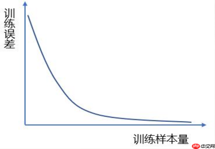
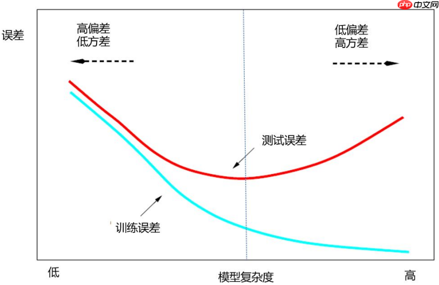
训练误差的大小与模型复杂度和训练样本量有关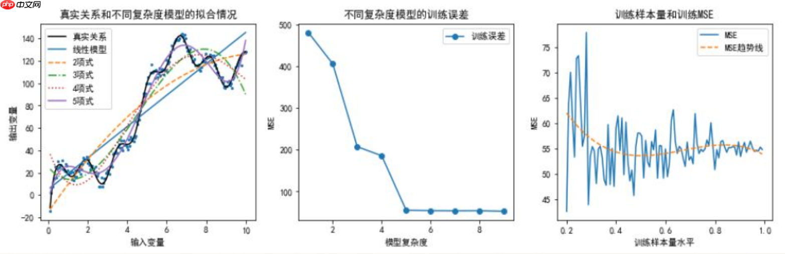
训练样本量和训练误差的理论关系
泛化误差的估计:泛化误差是无法直接计算的
ErrT=E[L(yi,hatf(Xi))∣T]=Ntest1i=1∑Ntest(yi−yi^)2 Err=E[L(yi,f^(Xi))]=E[ErrT]
训练误差和测试误差的关系(单次随机划分和多次随机划分的情况)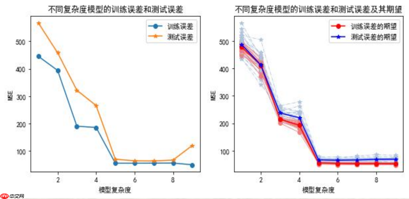
代码实现如下:
# 训练误差的大小与模型复杂度和训练样本量的关系图像# 导入所需模块import numpy as npimport pandas as pdimport matplotlib.pyplot as plt
%matplotlib inline# 解决中文乱码问题plt.rcParams['font.sans-serif']=['FZHuaLi-M14S']
plt.rcParams['axes.unicode_minus'] = Falseimport warnings
warnings.filterwarnings(action = 'ignore')from sklearn.metrics import confusion_matrix,f1_score,roc_curve, auc, precision_recall_curve,accuracy_scorefrom sklearn.model_selection import train_test_split,KFold,LeaveOneOut,LeavePOut # 数据集划分方法from sklearn.model_selection import cross_val_score,cross_validate # 计算交叉验证下的测试误差from sklearn import preprocessingimport sklearn.linear_model as LMfrom sklearn import neighbors


np.random.seed(123)
N=200x=np.linspace(0.1,10, num=N)
y=[]
z=[]for i in range(N):
    tmp=10*np.math.sin(4*x[i])+10*x[i]+20*np.math.log(x[i])+30*np.math.cos(x[i])
    y.append(tmp)
    tmp=y[i]+np.random.normal(0,3)
    z.append(tmp)

fig,axes=plt.subplots(nrows=1,ncols=3,figsize=(15,4))
axes[0].scatter(x,z,s=5)
axes[0].plot(x,y,'k-',label="真实关系")

modelLR=LM.LinearRegression()
X=x.reshape(N,1)
Y=np.array(z)
modelLR.fit(X,Y)
axes[0].plot(x,modelLR.predict(X),label="线性模型")
linestyle=['--','-.',':','-']for i in np.arange(1,5):
    tmp=pow(x,(i+1)).reshape(N,1)
    X=np.hstack((X,tmp))
    modelLR.fit(X,Y)
    axes[0].plot(x,modelLR.predict(X),linestyle=linestyle[i-1],label=str(i+1)+"项式")
axes[0].legend()
axes[0].set_title("真实关系和不同复杂度模型的拟合情况")
axes[0].set_xlabel("输入变量")
axes[0].set_ylabel("输出变量")

X=x.reshape(N,1)
Y=np.array(z)
modelLR.fit(X,Y)
MSEtrain=[np.sum((Y-modelLR.predict(X))**2)/(N-2)]for i in np.arange(1,9):
    tmp=pow(x,(i+1)).reshape(N,1)
    X=np.hstack((X,tmp))
    modelLR.fit(X,Y)
    MSEtrain.append(np.sum((Y-modelLR.predict(X))**2)/(N-(i+2)))
axes[1].plot(np.arange(1,10),MSEtrain,marker='o',label='训练误差')
axes[1].legend()
axes[1].set_title("不同复杂度模型的训练误差")
axes[1].set_xlabel("模型复杂度")
axes[1].set_ylabel("MSE")

X=x.reshape(N,1)
Y=np.array(z)for i in np.arange(1,5):  #采用5项式模型
    tmp=pow(x,(i+1)).reshape(N,1)
    X=np.hstack((X,tmp))
np.random.seed(0)
size=np.linspace(0.2,0.99,100)
MSEtrain=[]for i in range(len(size)):
    Ntraining=int(N*size[i])    id=np.random.choice(N,Ntraining,replace=False)
    X_train=X[id]
    y_train=Y[id]
    modelLR.fit(X_train,y_train)
    MSEtrain.append(np.sum((y_train-modelLR.predict(X_train))**2)/(Ntraining-6))

tmpx=np.linspace(1,len(size), num=len(size)).reshape(len(size),1)  #拟合MSEtmpX=np.hstack((tmpx,tmpx**2))
tmpX=np.hstack((tmpX,tmpx**3))
modelLR.fit(tmpX,MSEtrain)

axes[2].plot(size,MSEtrain,linewidth=1.5,linestyle='-',label='MSE')
axes[2].plot(size,modelLR.predict(tmpX),linewidth=1.5,linestyle='--',label='MSE趋势线')
axes[2].set_title("训练样本量和训练MSE")
axes[2].set_xlabel("训练样本量水平")
axes[2].set_ylabel("MSE")
axes[2].legend()
plt.show()<Figure size 1500x400 with 3 Axes>
说明:
1、这里通过数据模拟直观展示模型复杂度和训练误差的关系。随模型复杂度的提高,训练误差单调下降。
2、首先设定输入变量和输出变量的真实关系,并通过加上服从正态分布的随机数模拟其他随机因素对输出变量的影响。这里,设定的真实关系函数可以被泰勒展开,因此一定是次数越高的多项式模型越贴近真实观测值。 到达一定阶数(这里为9)后继续增加阶数对参数估计结果的影响很小可以忽略,无需再增加阶数。
3、分别建立各个多项式模型。这里消除了模型复杂度本身导致对MSE计算结果的影响,MSE计算时分母为自由度:样本量-(输入变量个数+1)。
4、考察训练集样本量对对于特定模型(这里为五项式)学习充分性的影响。样本量依次为原数据集的20%至99%。这里消除了样本量本身对MSE计算结果的影响,MSE计算时分母为自由度:样本量-(输入变量个数+1)。对不同样本量下的MSE进行三次曲线拟合。
# 训练误差和测试误差的关系图像fig,axes=plt.subplots(nrows=1,ncols=2,figsize=(10,4))
modelLR=LM.LinearRegression()

np.random.seed(123)
Ntraining=int(N*0.7)
Ntest=int(N*0.3)id=np.random.choice(N,Ntraining,replace=False)
X_train=x[id].reshape(Ntraining,1)
y_train=np.array(z)[id].reshape(Ntraining,1)
modelLR.fit(X_train,y_train)
MSEtrain=[np.sum((y_train-modelLR.predict(X_train))**2)/(Ntraining-2)]

xtest= np.delete(x, id).reshape(Ntest,1)
X_test= np.delete(x, id).reshape(Ntest,1)
y_test=np.delete(z,id).reshape(Ntest,1)
MSEtest=[np.sum((y_test-modelLR.predict(X_test))**2)/(Ntest-2)]for i in np.arange(1,9):
    tmp=pow(x[id],(i+1)).reshape(Ntraining,1)
    X_train=np.hstack((X_train,tmp))
    modelLR.fit(X_train,y_train)
    MSEtrain.append(np.sum((y_train-modelLR.predict(X_train))**2)/(Ntraining-(i+2)))
    tmp=pow(xtest,(i+1)).reshape(Ntest,1)
    X_test=np.hstack((X_test,tmp))
    MSEtest.append(np.sum((y_test-modelLR.predict(X_test))**2)/(Ntest-(i+2)))

axes[0].plot(np.arange(1,10,1),MSEtrain,marker='o',label='训练误差')
axes[0].plot(np.arange(1,10,1),MSEtest,marker='*',label='测试误差')
axes[0].legend()
axes[0].set_title("不同复杂度模型的训练误差和测试误差")
axes[0].set_xlabel("模型复杂度")
axes[0].set_ylabel("MSE")

MSEtrain=[]
MSEtest=[]for j in range(20):
    x=np.linspace(0.1,10, num=N)    id=np.random.choice(N,Ntraining,replace=False)
    X_train=x[id].reshape(Ntraining,1)
    y_train=np.array(z)[id].reshape(Ntraining,1)
    modelLR.fit(X_train,y_train)
    mse_train=[np.sum((y_train-modelLR.predict(X_train))**2)/(Ntraining-2)]

    xtest= np.delete(x, id).reshape(Ntest,1)
    X_test= np.delete(x, id).reshape(Ntest,1)
    y_test=np.delete(z,id).reshape(Ntest,1)
    mse_test=[np.sum((y_test-modelLR.predict(X_test))**2)/(Ntest-2)]    for i in np.arange(1,9):
        tmp=pow(x[id],(i+1)).reshape(Ntraining,1)
        X_train=np.hstack((X_train,tmp))
        modelLR.fit(X_train,y_train)
        mse_train.append(np.sum((y_train-modelLR.predict(X_train))**2)/(Ntraining-(i+2)))
        tmp=pow(xtest,(i+1)).reshape(Ntest,1)
        X_test=np.hstack((X_test,tmp))
        mse_test.append(np.sum((y_test-modelLR.predict(X_test))**2)/(Ntest-(i+2)))
    plt.plot(np.arange(1,10),mse_train,marker='o',linewidth=0.8,c='lightcoral',linestyle='-')
    plt.plot(np.arange(1,10),mse_test,marker='*',linewidth=0.8,c='lightsteelblue',linestyle='-.')
    MSEtrain.append(mse_train)
    MSEtest.append(mse_test)

MSETrain=pd.DataFrame(MSEtrain)
MSETest=pd.DataFrame(MSEtest)
axes[1].plot(np.arange(1,10),MSETrain.mean(),marker='o',linewidth=1.5,c='red',linestyle='-',label="训练误差的期望")
axes[1].plot(np.arange(1,10),MSETest.mean(),marker='*',linewidth=1.5,c='blue',linestyle='-',label="测试误差的期望")
axes[1].set_title("不同复杂度模型的训练误差和测试误差及其期望")
axes[1].set_xlabel("模型复杂度")
axes[1].set_ylabel("MSE")
axes[1].legend()
plt.show()<Figure size 1000x400 with 2 Axes>
说明:
1、这里通过数据模拟直观展示不同复杂度模型下训练误差和测试误差的关系。随模型复杂度的提高,训练误差单调下降,测试误差呈先下降后来上升的U字形。
2、从数据集中随机抽取一定比例的样本观测组成训练集训练模型,剩余的样本观测组成测试集计算测试误差。这里进行了20次。
3、样本观测的随机抽取必然导致20个训练集包含可能不同的样本观测,由此模型的参数估计值会有差别,从而使得20个训练误差和测试误差的数值结果不尽相等。带圆点的浅红色和浅灰色分别对应20次抽样的训练误差和测试误差,它们各自的均值对应带星号的红色和蓝色线。
CV(f^,α)=N1i=1∑NL(yi,f^−k(i)(Xi,α))
- $\alpha$表示人为指定的数据集划分策略。$\alpha$不同所导致的训练集不同将最终体现在预测模型上,因此将预测模型记为:$\hat{f}^{-k}(X,\alpha)$,表示第$\alpha$个预测模型(基于删去$k$部分数据之外的数据)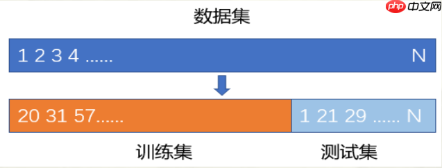
# 旁置法和留一法np.random.seed(123)
N=200x=np.linspace(0.1,10, num=N)
y=[]
z=[]for i in range(N):
tmp=10*np.math.sin(4*x[i])+10*x[i]+20*np.math.log(x[i])+30*np.math.cos(x[i])
y.append(tmp)
tmp=y[i]+np.random.normal(0,3)
z.append(tmp)
X=x.reshape(N,1)
Y=np.array(z)for i in np.arange(1,5): #采用5项式模型
tmp=pow(x,(i+1)).reshape(N,1)
X=np.hstack((X,tmp))
X_train, X_test, Y_train, Y_test = train_test_split(X,Y,train_size=0.70, random_state=123) #旁置法print("旁置法的训练集:%s ;测试集:%s" % (X_train.shape,X_test.shape))
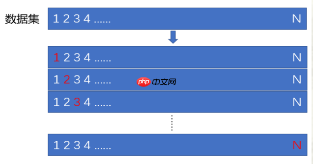
loo = LeaveOneOut() #留一法for train_index, test_index in loo.split(X): print("留一法训练集的样本量:%s;测试集的样本量: %s" % (len(train_index), len(test_index))) breaklpo = LeavePOut(p=3) # 留p法for train_index, test_index in lpo.split(X): print("留p法训练集的样本量:%s;测试集的样本量: %s" % (len(train_index),len(test_index)))
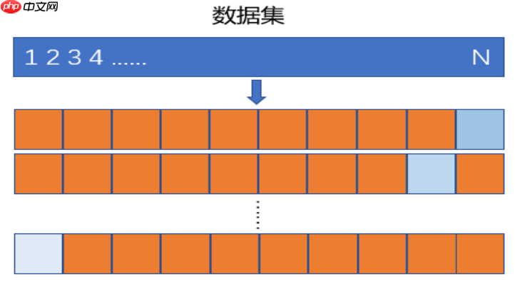
breakkf = KFold(n_splits=5,shuffle=True,random_state=123) # K折交叉验证法for train_index, test_index in kf.split(X): #给出索引
print("5折交叉验证法的训练集:",train_index,"\n测试集:",test_index) break旁置法的训练集:(140, 5) ;测试集:(60, 5) 留一法训练集的样本量:199;测试集的样本量: 1 留p法训练集的样本量:197;测试集的样本量: 3 5折交叉验证法的训练集: [ 0 1 2 3 5 6 7 8 9 10 11 12 13 14 15 16 17 18 21 22 23 24 25 27 28 29 30 32 33 34 35 36 38 39 40 41 42 43 44 45 46 47 48 49 51 54 55 56 57 58 59 60 61 62 63 64 65 66 67 68 69 70 71 73 74 75 76 77 78 80 81 83 84 86 87 89 90 91 92 94 96 97 98 99 100 101 102 103 105 106 107 109 110 111 112 113 114 115 116 117 118 120 122 123 124 125 126 129 130 131 132 134 135 136 137 138 141 142 143 145 146 147 148 150 151 152 153 154 155 156 157 159 160 161 163 164 165 167 168 169 171 173 174 175 176 177 181 186 187 188 190 191 192 193 194 195 196 197 198 199] 测试集: [ 4 19 20 26 31 37 50 52 53 72 79 82 85 88 93 95 104 108 119 121 127 128 133 139 140 144 149 158 162 166 170 172 178 179 180 182 183 184 185 189]
说明:
1、这里利用前述模拟数据,考察三种数据集划分及其测试误差的计算结果。需要引用sklearn.model_selection中的相关函数。
2、train_test_split(X,Y,train_size=0.70, random_state=123)实现数据集(X为输入变量矩阵,包含5个输入变量。输出变量为Y)划分的旁置法,这里指定训练集占原数据集(样本量为200)的70%,剩余30%为测试集。可指定random_state为任意整数以确保数据集的随机划分结果可以重现。函数依次返回训练集和测试集的输入变量和输出变量。可以看到划分结果为:训练集:(140, 5) ;测试集:(60, 5)。
3、LeaveOneOut()实现留一法,可利用结果对象的split方法,浏览数据集的划分结果,即训练集和测试集的样本观测索引(编号)。因原数据集样本量为200,留一法将做200次训练集和测试集的轮换,可利用循环浏览每次的划分结果。这里利用break跳出循环,只看第1次的划分结果。LeavePOut(p=3)是对留一法的拓展,为留p法。例如这里测试集的样本量为3。
4、KFold(n_splits=5,shuffle=True,random_state=123)实现K折交叉验证法,这里为k=5。指定shuffle=True表示将数据顺序随机打乱后再做K折划分。这里仅显示了1次划分的结果(样本观测索引)。
# K折交叉验证modelLR=LM.LinearRegression()
k=10CVscore=cross_val_score(modelLR,X,Y,cv=k,scoring='neg_mean_squared_error')   #sklearn.metrics.SCORERS.keys()print("k=10折交叉验证的MSE:",-1*CVscore.mean())
scores = cross_validate(modelLR,X,Y, scoring='neg_mean_squared_error',cv=k, return_train_score=True)print("k=10折交叉验证的MSE:",-1*scores['test_score'].mean())  # scores为字典#N折交叉验证:LOOCVscore=cross_val_score(modelLR,X,Y,cv=N,scoring='neg_mean_squared_error')
print("LOO的MSE:",-1*CVscore.mean())k=10折交叉验证的MSE: 103.51193551457445 k=10折交叉验证的MSE: 103.51193551457445 LOO的MSE: 56.84058776221936
说明:cross_val_score()和cross_validate()都可自动给出模型在K折交叉验证法下的测试误差,cross_validate还可给出训练误差。这里,模型为一般线性回归模型(五项式模型),计算10折交叉验证法下的测试误差。参数scoring为模型预测精度的度量,指定特定字符串,计算相应评价指标的结果。例如:'neg_mean_squared_error'表示计算负的MSE。可通过sklearn.metrics.SCORERS.keys()浏览其他的评价指标。若指定参数cv等于样本量,可得到N折交叉验证法(即留一法LOO)下的测试误差。
模型选择的基本原则
预测模型中的“佼佼者”应具有两个重要特征:
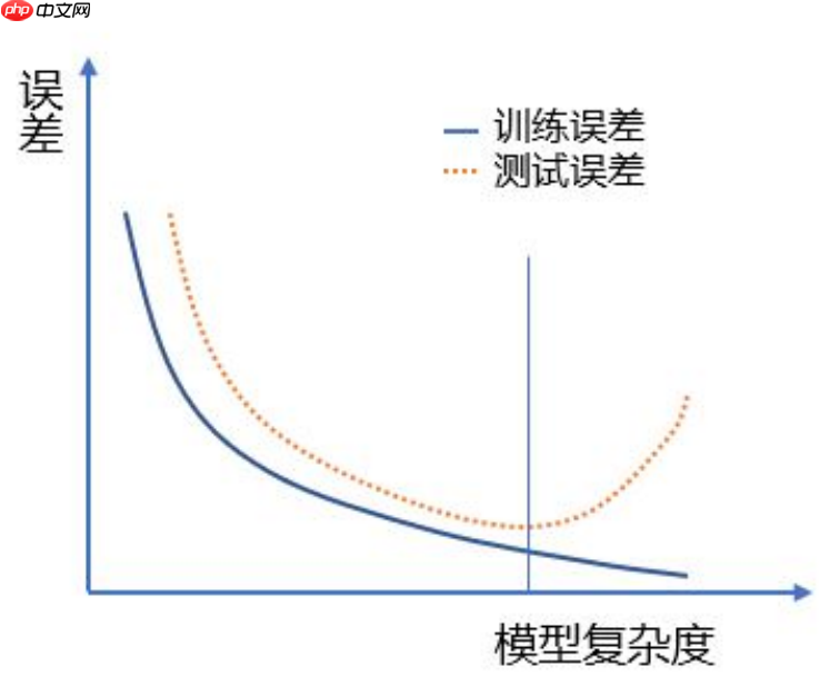
选择复杂模型将导致怎样的后果?
模型过拟合
# 各种情况下的拟合np.random.seed(123)
N=100x=np.linspace(-10,10, num=N)
y=14+5.5*x+4.8*x**2+0.5*x**3z=[]for i in range(N):
    z.append(y[i]+np.random.normal(0,50))

fig,axes=plt.subplots(nrows=1,ncols=2,figsize=(10,4))
axes[0].scatter(x,z,s=10)
axes[0].plot(x,y,'k-',label="真实关系")
modelLR=LM.LinearRegression()
X=x.reshape(N,1)
Y=np.array(z)
modelLR.fit(X,Y)
axes[0].plot(x,modelLR.predict(X),linestyle='--',label="线性模型")
linestyle=[':','-.']
degree=[2,3]for i in range(len(degree)):
    tmp=pow(x,degree[i]).reshape(N,1)
    X=np.hstack((X,tmp))
    modelLR.fit(X,Y)
    axes[0].plot(x,modelLR.predict(X),linestyle=linestyle[i],label=str(degree[i])+"项式模型")
KNNregr=neighbors.KNeighborsRegressor(n_neighbors=5)
X=x.reshape(N,1)
KNNregr.fit(X,Y)
axes[0].plot(X,KNNregr.predict(X),linestyle='-',label="复杂模型")
axes[0].legend()
axes[0].set_title("真实关系和不同复杂度模型的拟合情况")
axes[0].set_xlabel("输入变量")
axes[0].set_ylabel("输出变量")

X=x.reshape(N,1)
Y=np.array(z)
modelLR.fit(X,Y)
np.random.seed(123)
k=10scores = cross_validate(modelLR,X,Y, scoring='neg_mean_squared_error',cv=k, return_train_score=True)
MSEtrain=[-1*scores['train_score'].mean()]
MSEtest=[-1*scores['test_score'].mean()]
degree=[2,3]for i in range(len(degree)):
    tmp=pow(x,degree[i]).reshape(N,1)
    X=np.hstack((X,tmp))
    modelLR.fit(X,Y)
    scores = cross_validate(modelLR,X,Y, scoring='neg_mean_squared_error',cv=k, return_train_score=True)
    MSEtrain.append((-1*scores['train_score']).mean())
    MSEtest.append((-1*scores['test_score']).mean())

KNNregr=neighbors.KNeighborsRegressor(n_neighbors=5)
X=x.reshape(N,1)
KNNregr.fit(X,Y)
scores = cross_validate(KNNregr,X,Y, scoring='neg_mean_squared_error',cv=k, return_train_score=True)
MSEtrain.append((-1*scores['train_score']).mean())
MSEtest.append((-1*scores['test_score']).mean())

axes[1].plot(np.arange(1,len(degree)+3),MSEtrain,marker='o',label='训练误差(10折交叉验证法)',linestyle='--')
axes[1].plot(np.arange(1,len(degree)+3),MSEtest,marker='*',label='测试误差(10折交叉验证法)')

axes[1].legend()
axes[1].set_title("不同复杂度模型的训练误差和测试误差(Err)")
axes[1].set_xlabel("模型复杂度")
axes[1].set_ylabel("MSE")
fig.show()<Figure size 1000x400 with 2 Axes>
说明:
1、利用通过数据模拟,直观展示模型的过拟合,以及过拟合模型下的训练误差和测试误差的特点。
2、这里,复杂模型为K近邻法建立的预测模型,是一种典型的非线性模型。具体内容详见第4章。
3、对不同复杂度模型,利用cross_validate()计算10折交叉验证下的训练误差和测试误差。随模型复杂度的提高,训练误差单调下降,测试误差呈先下降后来上升的U字形。显然,复杂模型的训练误差最小但测试误差并非最小,出现了模型的过拟合。
4、scores['train_score']为训练误差,scores['test_score']为测试误差。
# 4个模型10折交叉验证下各折测试误差的分布特征fig,axes = plt.subplots(1,2,figsize=(10,4))
modelLR=LM.LinearRegression()
X=x.reshape(N,1)
Y=np.array(z)
modelLR.fit(X,Y)
np.random.seed(123)
k=10scores = cross_validate(modelLR,X,Y, scoring='neg_mean_squared_error',cv=k, return_train_score=True)
fdata=pd.Series(-1*scores['test_score'])
axes[0].boxplot(x=fdata,sym='rd',patch_artist=True,boxprops={'color':'blue','facecolor':'pink'},labels ={"线性模型"},showfliers=False)
MSEMedian=[np.median(-1*scores['test_score'])]
MSEVar=[(-1*scores['test_score']).var()]
MSEMean=[(-1*scores['test_score']).mean()]

degree=[2,3]
lab=['二项式模型','三项式项模型']for i in range(len(degree)):
    tmp=pow(x,degree[i]).reshape(N,1)
    X=np.hstack((X,tmp))
    modelLR.fit(X,Y)
    scores = cross_validate(modelLR,X,Y, scoring='neg_mean_squared_error',cv=k, return_train_score=True)
    fdata=pd.Series(-1*scores['test_score'])
    axes[0].boxplot(x=fdata,sym='rd',positions=[i+2],patch_artist=True,boxprops={'color':'blue','facecolor':'pink'},labels ={lab[i]},
                    showfliers=False)
    MSEMedian.append(np.median(-1*scores['test_score']))
    MSEVar.append((-1*scores['test_score']).var())
    MSEMean.append((-1*scores['test_score']).mean())

KNNregr=neighbors.KNeighborsRegressor(n_neighbors=5)
X=x.reshape(N,1)
KNNregr.fit(X,Y)
scores = cross_validate(KNNregr,X,Y, scoring='neg_mean_squared_error',cv=k, return_train_score=True)
fdata=pd.Series(-1*scores['test_score'])
axes[0].boxplot(x=fdata,sym='rd',positions=[4],patch_artist=True,boxprops={'color':'blue','facecolor':'pink'},labels ={"复杂模型"},
                showfliers=False)
MSEMedian.append(np.median(-1*scores['test_score']))
MSEVar.append((-1*scores['test_score']).var())
MSEMean.append((-1*scores['test_score']).mean())

axes[0].plot(np.arange(1,5),MSEMedian,marker='o',linestyle='--')
axes[0].set_ylabel('MSE')
axes[0].set_xlabel('复杂度')
axes[0].set_title('不同复杂度模型下的Err(10折交叉验证法)')
axes[0].grid(linestyle="--", alpha=0.3)

axes[1].plot(np.arange(1,5),preprocessing.scale(MSEMean),marker='o',linestyle='-',label="Err")
axes[1].plot(np.arange(1,5),preprocessing.scale(MSEVar),marker='o',linestyle='--',label="方差")
axes[1].grid(linestyle="--", alpha=0.3)

axes[1].set_title('不同复杂度模型测试误差的期望(Err)与方差变化趋势图')
axes[1].set_xlabel('复杂度')
axes[1].set_ylabel('标准化值')
plt.legend(loc='best', bbox_to_anchor=(1, 1))<matplotlib.legend.Legend at 0x7ff742d9dc10>
<Figure size 1000x400 with 2 Axes>
说明:
1、对于上述模拟数据和四种复杂度模型,利用箱线图展示了10折交叉验证下各折测试误差的统计分布。简单模型预测误差大,表现出测试误差箱线图的中位数线偏高,均值大,且箱体宽方差较大。随着复杂度增加情况相应发生改变。
2、boxplot()画箱线图时可以指定多个箱体在图中的位置(positions),箱体是否填充色(patch_artist=True),并以数据字典方式指定箱体边框颜色('color':'blue')填充色('facecolor':'pink'),箱体标签(labels)以及是否显示数据中的异常点(showfliers)等。
3、preprocessing.scale()是对数据进行标准化处理,即数据减去均值除以标准差。处理后的数据均值等于0标准差等于1。通过标准化处理实现将不同数量级的数据变动趋势画在同一幅图中。
预测模型的偏差:
预测模型的方差:
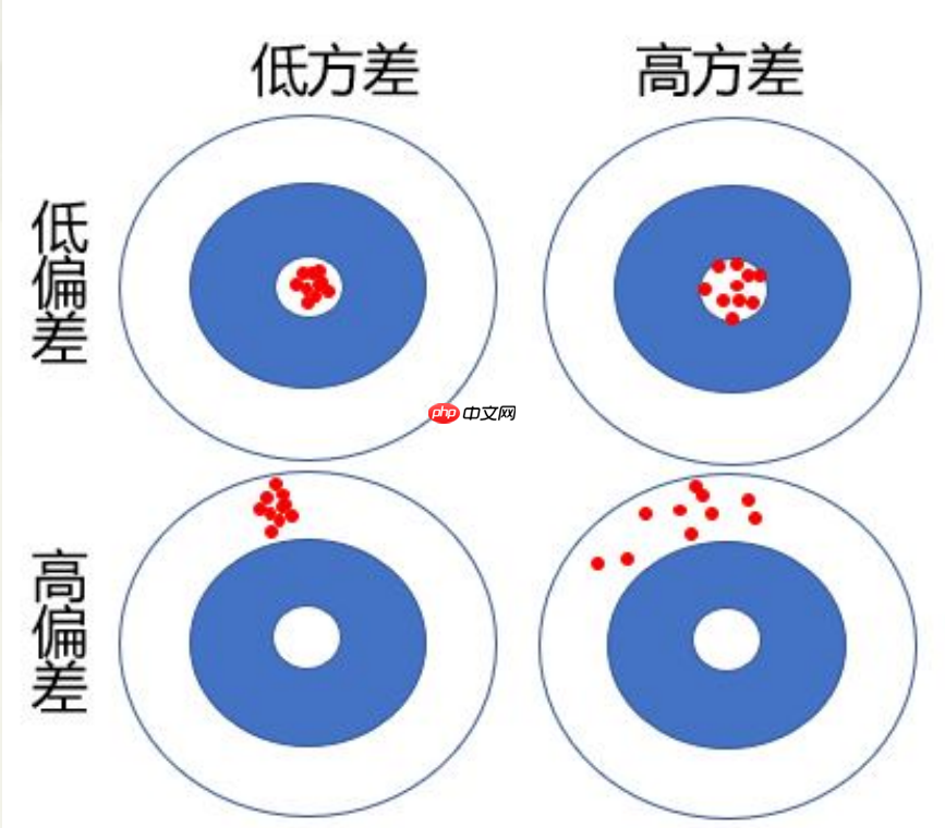
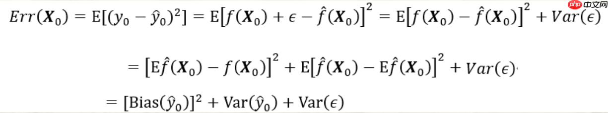
第三项为随机误差项的方差。无论怎样调整模型,第三项都不可能消失除非σε2=0;第一项为上述的偏差的平方,度量了预测值的平均值与真实值的差;第二项为上述的方差,度量了预测值与其期望间的平均性平方差异
# 预测模型的偏差和方差的变化趋势图x0=np.array([x.mean(),x.mean()**2,x.mean()**3])
y0=14+5.5*x0[0]+4.8*x0[1]+0.5*x0[2]
X=x.reshape(N,1)
Y=np.array(z)
degree=[2,3]for i in range(len(degree)):
    tmp=pow(x,degree[i]).reshape(N,1)
    X=np.hstack((X,tmp))
modelLR=LM.LinearRegression()
KNNregr=neighbors.KNeighborsRegressor(n_neighbors=5)
model1,model2,model3,model4=[],[],[],[]
kf = KFold(n_splits=10,shuffle=True,random_state=123)for train_index, test_index in kf.split(X):
    Ntrain=len(train_index)
    XKtrain=X[train_index,]
    YKtrain=Y[train_index,]
    modelLR.fit(XKtrain[:,0].reshape(Ntrain,1),YKtrain)
    model1.append(modelLR.predict(x0[0].reshape(1,1)))
    modelLR.fit(XKtrain[:,0:2].reshape(Ntrain,2),YKtrain)
    model2.append(modelLR.predict(x0[0:2].reshape(1,2)))
    modelLR.fit(XKtrain[:,0:3].reshape(Ntrain,3),YKtrain)
    model3.append(modelLR.predict(x0[0:3].reshape(1,3)))
    KNNregr.fit(XKtrain[:,0].reshape(Ntrain,1),YKtrain)
    model4.append(KNNregr.predict(x0[0].reshape(1,1)))

fig,axes = plt.subplots(1,1,figsize=(6,4))
VI=[np.var(model1)/np.mean(model1),np.var(model2)/np.mean(model2),np.var(model3)/np.mean(model3),np.var(model4)//np.mean(model4)]
Err=[np.mean(model1)-y0,np.mean(model2)-y0,np.mean(model3)-y0,np.mean(model4)-y0]
Err=pow(np.array(Err),2)

axes.plot(np.arange(1,5),preprocessing.scale(VI),marker='o',linestyle='-',label='方差')
axes.plot(np.arange(1,5),preprocessing.scale(Err),marker='o',linestyle='--',label='偏差')
axes.plot(np.arange(1,5),preprocessing.scale(MSEMean),marker='o',linestyle='-.',label="Err")
axes.set_ylabel('标准化值')
axes.set_xlabel('复杂度')
axes.set_title('不同复杂度模型的Err以及偏差和方差的变化趋势图')
axes.grid(linestyle="--", alpha=0.3)
plt.legend(loc='center',bbox_to_anchor=(0.5,0.8))
fig.show()<Figure size 600x400 with 1 Axes>
data=pd.read_excel('北京市空气质量数据.xlsx')
data=data.replace(0,np.NaN)
data=data.dropna()
data['有无污染']=data['质量等级'].map({'优':0,'良':0,'轻度污染':1,'中度污染':1,'重度污染':1,'严重污染':1})print(data['有无污染'].value_counts())
fig = plt.figure()
ax = fig.add_subplot(111)
flag=(data['有无污染']==0)
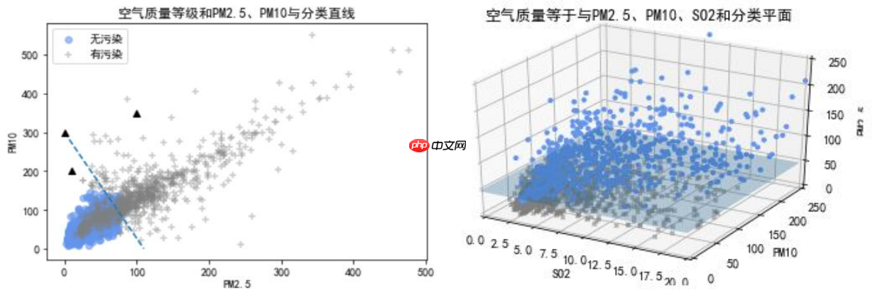
ax.scatter(data.loc[flag,'PM2.5'],data.loc[flag,'PM10'],c='cornflowerblue',marker='o',label='无污染',alpha=0.6)
flag=data['有无污染']==1ax.scatter(data.loc[flag,'PM2.5'],data.loc[flag,'PM10'],c='grey',marker='+',label='有污染',alpha=0.4)
ax.set_xlabel('PM2.5')
ax.set_ylabel('PM10')
plt.legend()##Logistic回归X=data[['PM2.5','PM10']]
y=data['有无污染']
modelLR=LM.LogisticRegression()
modelLR.fit(X,y)print("截距项:%f"%modelLR.intercept_)print("回归系数:",modelLR.coef_)print("优势比{0}".format(np.exp(modelLR.coef_)))
yhat=modelLR.predict(X)print("预测结果:",yhat)print("总的错判率:%f"%(1-modelLR.score(X,y)))0 1204 1 892 Name: 有无污染, dtype: int64 截距项:-4.858429 回归系数: [[0.05260358 0.01852681]] 优势比[[1.05401173 1.0186995 ]] 预测结果: [0 1 0 ... 0 0 0] 总的错判率:0.153149
<Figure size 640x480 with 1 Axes>
说明:
1、这里以空气质量监测数据为例,对是否有污染(二分类输出变量)进行预测。首先对数据进行预处理,将质量等级是优和良的合并为0类(无污染)共计1204天。其余合并为1类(有污染)共计892天。这里只考虑PM2.5和PM10对有无污染的影响,作为输入变量,只有0和1两个取值的有无污染作为输出变量。建立Logistic回归模型。
2、首先,modelLR=LM.LogisticRegression()定义modelLR对象为Logistic回归模型;然后,modelLR.fit(X,y)表示基于给出的X和y估计模型参数。其中,X为输入变量(矩阵形式),y为输出变量。
3、模型参数的估计值存储在intercept_和.coef_属性中,依次为截距项和回归系数。从回归系数估计值看,PM2.5(系数为0.05)对是否有污染的作用比PM10(系数为0.02)更大。
4、modelLR.predict(X)表示将X带入回归方程计算y的预测值。
X=data.loc[:,['PM2.5','PM10','SO2','CO','NO2','O3']]
Y=data.loc[:,'有无污染']
modelLR=LM.LogisticRegression()
modelLR.fit(X,Y)print('训练误差:',1-modelLR.score(X,Y))  #print(accuracy_score(Y,modelLR.predict(X)))print('混淆矩阵:\n',confusion_matrix(Y,modelLR.predict(X)))print('F1-score:',f1_score(Y,modelLR.predict(X),pos_label=1))
fpr,tpr,thresholds = roc_curve(Y,modelLR.predict_proba(X)[:,1],pos_label=1) ###计算fpr和tprroc_auc = auc(fpr,tpr) ###计算auc的值print('AUC:',roc_auc)print('总正确率',accuracy_score(Y,modelLR.predict(X)))
fig,axes=plt.subplots(nrows=1,ncols=2,figsize=(10,4))
axes[0].plot(fpr, tpr, color='r',linewidth=2, label='ROC curve (area = %0.5f)' % roc_auc)
axes[0].plot([0, 1], [0, 1], color='navy', linewidth=2, linestyle='--')
axes[0].set_xlim([-0.01, 1.01])
axes[0].set_ylim([-0.01, 1.01])
axes[0].set_xlabel('FPR')
axes[0].set_ylabel('TPR')
axes[0].set_title('ROC曲线')
axes[0].legend(loc="lower right")

pre, rec, thresholds = precision_recall_curve(Y,modelLR.predict_proba(X)[:,1],pos_label=1)
axes[1].plot(rec, pre, color='r',linewidth=2, label='总正确率 = %0.3f)' % accuracy_score(Y,modelLR.predict(X)))
axes[1].plot([0,1],[1,pre.min()],color='navy', linewidth=2, linestyle='--')
axes[1].set_xlim([-0.01, 1.01])
axes[1].set_ylim([pre.min()-0.01, 1.01])
axes[1].set_xlabel('查全率R')
axes[1].set_ylabel('查准率P')
axes[1].set_title('P-R曲线')
axes[1].legend(loc='lower left')
plt.show()训练误差: 0.0782442748091603 混淆矩阵: [[1128 76] [ 88 804]] F1-score: 0.90744920993228 AUC: 0.982303010890455 总正确率 0.9217557251908397
<Figure size 1000x400 with 2 Axes>
说明:
1、这里利用空气质量监测数据,建立Logistic回归模型对是否有污染进行分类预测。其中的输入变量包括PM2.5,PM10,SO2,CO,NO2,O3污染物浓度,是否有污染为二分类的输出变量(1为有污染,0为无污染)。进一步,对模型进行评价,涉及ROC曲线、AUC值以及F1分数等。需引用sklearn.metrics中的confusion_matrix,f1_score,roc_curve, auc,以及import accuracy_score等。
2、modelLR.score(X,Y)为预测模型的精度得分(基于训练集的)。分类预测的精度得分为总的预测正确率。也可通过accuracy_score函数得到同样结果。
3、confusion_matrix(Y,modelLR.predict(X)):计算模型的混淆矩阵。
4、f1_score(Y,modelLR.predict(X),pos_label=1):针对1类计算F1得分。
5、modelLR.predict_proba(X)中存储模型预测为0类和1类的概率,这里关心预测为1类的概率。
6、roc_curve:计算预测为1类的概率从大到小过程中的TPR和FPR。auc(fpr,tpr) 计算ROC曲线下的面积。
7、precision_recall_curve:计算预测为1类的概率从大到小过程中的查准率P和查全率R.
8、ROC曲线和AUC值,以及P-R曲线均表明,该预测模型的预测误差(训练误差)很小。
以上就是python机器学习数据建模与分析——数据预测与预测建模的详细内容,更多请关注php中文网其它相关文章!

python怎么学习?python怎么入门?python在哪学?python怎么学才快?不用担心,这里为大家提供了python速学教程(入门到精通),有需要的小伙伴保存下载就能学习啦!

Copyright 2014-2025 //m.sbmmt.com/ All Rights Reserved | php.cn | 湘ICP备2023035733号


 906
906