低通濾波器(Low Pass Filter, LPF) 過濾了影像中的高頻部分,並僅允許低頻部分通過。因此,在影像上套用LPF 會刪除影像中的細節/邊緣和雜訊/離群值,此過程也稱為影像模糊(或平滑),影像平滑可以作為複雜影像處理任務的預處理部分。
影像模糊通常包含以下類型:
邊緣模糊(Edge) 這種類型的模糊通常透過卷積明確地應用於影像,例如線性濾波器核或高斯核等,使用這些濾波器核可以平滑/去除影像中不必要的細節/雜訊。
動作模糊 (Motion) 通常是因為相機在拍攝影像時會抖動所產生的,也就是說,攝影機或被拍攝的物件處於移動狀態。我們可以使用點擴展函數來模擬這種模糊。
失焦模糊(de-focus) 當相機拍攝的物件失焦時,會產生這種類型的模糊;我們可以使用模糊(blur) 核來模擬這種模糊。
接下來,我們建立以上三種不同類型的核,並將它們應用於影像以觀察不同類型核處理影像後的結果。
(1) 我們先定義函數get_gaussian_edge_blur_kernel() 以傳回2D高斯模糊核用於邊緣模糊。此函數接受高斯標準差( σ σ σ) 以及創建2D 核的大小(例如,sz = 15 將建立尺寸為15x15 的核)作為函數的參數。如下所示,首先建立了一個1D 高斯核,然後計算兩個1D 高斯核的外積回傳2D 核:
import numpy as np
import numpy.fft as fp
from skimage.io import imread
from skimage.color import rgb2gray
import matplotlib.pyplot as plt
import cv2

def get_gaussian_edge_blur_kernel(sigma, sz=15):
    # First create a 1-D Gaussian kernel
    x = np.linspace(-10, 10, sz)
    kernel_1d = np.exp(-x**2/sigma**2)
    kernel_1d /= np.trapz(kernel_1d) # normalize the sum to 1.0
    # create a 2-D Gaussian kernel from the 1-D kernel
    kernel_2d = kernel_1d[:, np.newaxis] * kernel_1d[np.newaxis, :]
return kernel_2d(2) 接下來,定義函數get_motion_blur_kernel() 以產生運動模糊核,得到給定長度且特定方向(角度)的線作為卷積核,以模擬輸入影像的運動模糊效果:
def get_motion_blur_kernel(ln, angle, sz=15):
    kern = np.ones((1, ln), np.float32)
    angle = -np.pi*angle/180
    c, s = np.cos(angle), np.sin(angle)
    A = np.float32([[c, -s, 0], [s, c, 0]])
    sz2 = sz // 2
    A[:,2] = (sz2, sz2) - np.dot(A[:,:2], ((ln-1)*0.5, 0))
    kern = cv2.warpAffine(kern, A, (sz, sz), flags=cv2.INTER_CUBIC)
return kern函數get_motion_blur_kernel() 將模糊的長度和角度以及模糊核的尺寸作為參數,函數使用OpenCV 的 warpaffine() 函數傳回核矩陣(以矩陣中心為中點,使用給定長度和給定角度得到核)。
(3) 最後,定義函數get_out_of_focus_kernel() 以產生失焦核(模擬影像失焦模糊),其根據給定半徑建立圓形用作卷積核,函數接受半徑R (Deocus Radius) 和要產生的核大小作為輸入參數:
 def get_out_of_focus_kernel(r, sz=15):
    kern = np.zeros((sz, sz), np.uint8)
    cv2.circle(kern, (sz, sz), r, 255, -1, cv2.LINE_AA, shift=1)
    kern = np.float32(kern) / 255
return kern(4) 接下來,實作函數dft_convolve(),該函數使用影像的逐元素乘法和頻域中的捲積核執行頻域卷積(基於卷積定理)。函數也繪製輸入影像、核和卷積計算後得到的輸出影像:
def dft_convolve(im, kernel):
    F_im = fp.fft2(im)
    #F_kernel = fp.fft2(kernel, s=im.shape)
    F_kernel = fp.fft2(fp.ifftshift(kernel), s=im.shape)
    F_filtered = F_im * F_kernel
    im_filtered = fp.ifft2(F_filtered)
    cmap = 'RdBu'
    plt.figure(figsize=(20,10))
    plt.gray()
    plt.subplot(131), plt.imshow(im), plt.axis('off'), plt.title('input image', size=10)
    plt.subplot(132), plt.imshow(kernel, cmap=cmap), plt.title('kernel', size=10)
    plt.subplot(133), plt.imshow(im_filtered.real), plt.axis('off'), plt.title('output image', size=10)
    plt.tight_layout()
plt.show()(5) 將get_gaussian_edge_blur_kernel() 核函數套用至影像,並繪製輸入,核和輸出模糊圖像:
im = rgb2gray(imread('3.jpg'))

kernel = get_gaussian_edge_blur_kernel(25, 25)
dft_convolve(im, kernel)
(6) 接下來,將get_motion_blur_kernel() 函數應用於圖像,並繪製輸入,核和輸出模糊影像:
kernel = get_motion_blur_kernel(30, 60, 25)
dft_convolve(im, kernel)
(7) 最後,將get_out_of_focus_kernel() 函數套用至影像,並繪製輸入,核和輸出模糊影像:
kernel = get_out_of_focus_kernel(15, 20)
dft_convolve(im, kernel)
scipy.ndimage 模組提供了一系列可以在頻域中對圖像應用低通濾波器的函數。在本節中,我們透過幾個範例學習其中一些濾波器的用法。
使用scipy.ndimage 庫中的fourier_gaussian() 函數在頻域中使用高斯核執行卷積操作。
(1) 首先,讀取輸入影像,並將其轉換為灰階影像,並透過使用FFT 取得其頻域表示:
import numpy as np
import numpy.fft as fp
from skimage.io import imread
import matplotlib.pyplot as plt
from scipy import ndimage

im = imread('1.png', as_gray=True)
freq = fp.fft2(im)
(2) 接下來,使用fourier_gaussian() 函數對影像執行模糊操作,使用兩個具有不同標準差的高斯核,繪製輸入、輸出影像以及功率譜:
fig, axes = plt.subplots(2, 3, figsize=(20,15))
plt.subplots_adjust(0,0,1,0.95,0.05,0.05)
plt.gray() # show the filtered result in grayscale
axes[0, 0].imshow(im), axes[0, 0].set_title('Original Image', size=10)
axes[1, 0].imshow((20*np.log10( 0.1 + fp.fftshift(freq))).real.astype(int)), axes[1, 0].set_title('Original Image Spectrum', size=10)
i = 1
for sigma in [3,5]:
    convolved_freq = ndimage.fourier_gaussian(freq, sigma=sigma)
    convolved = fp.ifft2(convolved_freq).real # the imaginary part is an artifact
    axes[0, i].imshow(convolved)
    axes[0, i].set_title(r'Output with FFT Gaussian Blur, $\sigma$={}'.format(sigma), size=10)
    axes[1, i].imshow((20*np.log10( 0.1 + fp.fftshift(convolved_freq))).real.astype(int))
    axes[1, i].set_title(r'Spectrum with FFT Gaussian Blur, $\sigma$={}'.format(sigma), size=10)
    i += 1
for a in axes.ravel():
    a.axis('off')
plt.show()scipy.ndimage 模組的函數fourier_uniform() 實作了多維均勻傅立葉濾波器。頻率陣列與給定尺寸的方形核的傅立葉變換相乘。接下來,我們學習如何使用 LPF (均值濾波器)模糊輸入灰階影像。
(1) 首先,讀取輸入影像並使用 DFT 取得其頻域表示:
im = imread('1.png', as_gray=True)
freq = fp.fft2(im)
(2) 然后,使用函数 fourier_uniform() 应用 10x10 方形核(由功率谱上的参数指定),以获取平滑输出:
freq_uniform = ndimage.fourier_uniform(freq, size=10)
(3) 绘制原始输入图像和模糊后的图像:
fig, (axes1, axes2) = plt.subplots(1, 2, figsize=(20,10))
plt.gray() # show the result in grayscale
im1 = fp.ifft2(freq_uniform)
axes1.imshow(im), axes1.axis('off')
axes1.set_title('Original Image', size=10)
axes2.imshow(im1.real) # the imaginary part is an artifact
axes2.axis('off')
axes2.set_title('Blurred Image with Fourier Uniform', size=10)
plt.tight_layout()
plt.show()
(4) 最后,绘制显示方形核的功率谱:
plt.figure(figsize=(10,10))
plt.imshow( (20*np.log10( 0.1 + fp.fftshift(freq_uniform))).real.astype(int))
plt.title('Frequency Spectrum with fourier uniform', size=10)
plt.show()
与上一小节类似,通过将方形核修改为椭圆形核,我们可以使用椭圆形核生成模糊的输出图像。
(1) 类似的,我们首先在图像的功率谱上应用函数 fourier_ellipsoid(),并使用 IDFT 在空间域中获得模糊后的输出图像:
freq_ellipsoid = ndimage.fourier_ellipsoid(freq, size=10)
im1 = fp.ifft2(freq_ellipsoid)
(2) 接下来,绘制原始输入图像和模糊后的图像:
fig, (axes1, axes2) = plt.subplots(1, 2, figsize=(20,10))
axes1.imshow(im), axes1.axis('off')
axes1.set_title('Original Image', size=10)
axes2.imshow(im1.real) # the imaginary part is an artifact
axes2.axis('off')
axes2.set_title('Blurred Image with Fourier Ellipsoid', size=10)
plt.tight_layout()
plt.show()
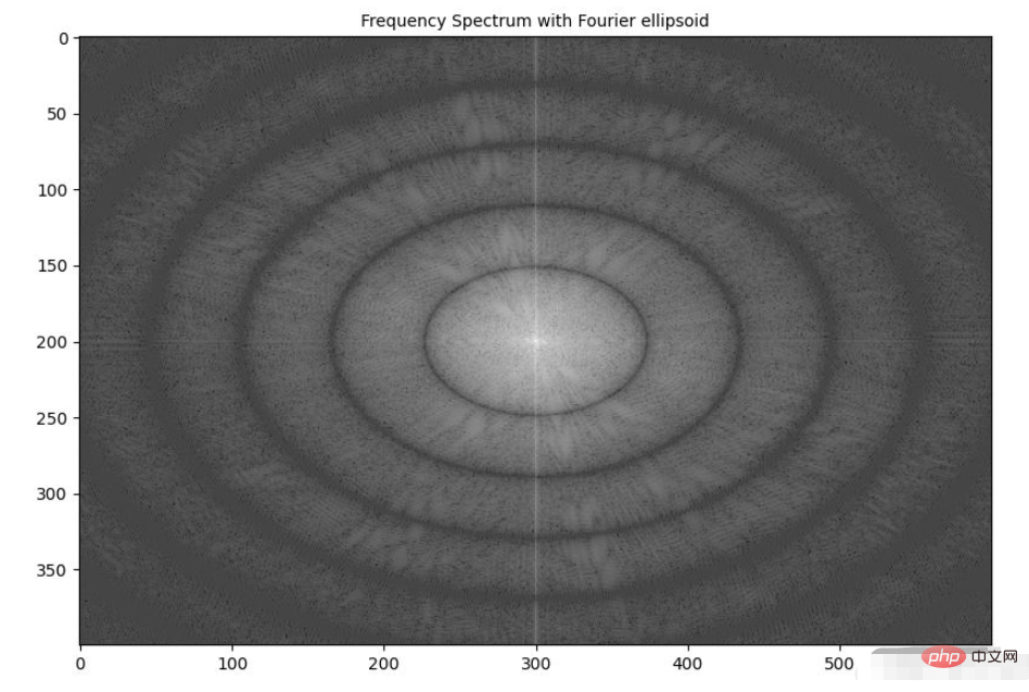
(3) 最后,显示应用椭圆形核后图像的频谱:
plt.figure(figsize=(10,10))
plt.imshow( (20*np.log10( 0.1 + fp.fftshift(freq_ellipsoid))).real.astype(int))
plt.title('Frequency Spectrum with Fourier ellipsoid', size=10)
plt.show()
我们已经学习了如何在实际应用中使用 numpy.fft 模块的 2D-FFT。在本节中,我们将介绍 scipy.fftpack 模块的 fft2() 函数用于实现高斯模糊。
(1) 使用灰度图像作为输入,并使用 FFT 从图像中创建 2D 频率响应数组:
import numpy as np
import numpy.fft as fp
from skimage.color import rgb2gray
from skimage.io import imread
import matplotlib.pyplot as plt
from scipy import signal
from matplotlib.ticker import LinearLocator, FormatStrFormatter

im = rgb2gray(imread('1.png'))
freq = fp.fft2(im)
(2) 通过计算两个 1D 高斯核的外积,在空间域中创建高斯 2D 核用作 LPF:
kernel = np.outer(signal.gaussian(im.shape[0], 1), signal.gaussian(im.shape[1], 1))
(3) 使用 DFT 获得高斯核的频率响应:
freq_kernel = fp.fft2(fp.ifftshift(kernel))
(4) 使用卷积定理通过逐元素乘法在频域中将 LPF 与输入图像卷积:
convolved = freq*freq_kernel # by the Convolution theorem
(5) 使用 IFFT 获得输出图像,需要注意的是,要正确显示输出图像,需要缩放输出图像:
im_blur = fp.ifft2(convolved).real
im_blur = 255 * im_blur / np.max(im_blur)
(6) 绘制图像、高斯核和在频域中卷积后获得图像的功率谱,可以使用 matplotlib.colormap 绘制色,以了解不同坐标下的频率响应值:
plt.figure(figsize=(20,20))
plt.subplot(221), plt.imshow(kernel, cmap='coolwarm'), plt.colorbar()
plt.title('Gaussian Blur Kernel', size=10)
plt.subplot(222)
plt.imshow( (20*np.log10( 0.01 + fp.fftshift(freq_kernel))).real.astype(int), cmap='inferno')
plt.colorbar()
plt.title('Gaussian Blur Kernel (Freq. Spec.)', size=10)
plt.subplot(223), plt.imshow(im, cmap='gray'), plt.axis('off'), plt.title('Input Image', size=10)
plt.subplot(224), plt.imshow(im_blur, cmap='gray'), plt.axis('off'), plt.title('Output Blurred Image', size=10)
plt.tight_layout()
plt.show()
(7) 要绘制输入/输出图像和 3D 核的功率谱,我们定义函数 plot_3d(),使用 mpl_toolkits.mplot3d 模块的 plot_surface() 函数获取 3D 功率谱图,给定相应的 Y 和Z值作为 2D 阵列传递:
def plot_3d(X, Y, Z, cmap=plt.cm.seismic):
    fig = plt.figure(figsize=(20,20))
    ax = fig.gca(projection='3d')
    # Plot the surface.
    surf = ax.plot_surface(X, Y, Z, cmap=cmap, linewidth=5, antialiased=False)
    #ax.plot_wireframe(X, Y, Z, rstride=10, cstride=10)
    #ax.set_zscale("log", nonposx='clip')
    #ax.zaxis.set_scale('log')
    ax.zaxis.set_major_locator(LinearLocator(10))
    ax.zaxis.set_major_formatter(FormatStrFormatter('%.02f'))
    ax.set_xlabel('F1', size=15)
    ax.set_ylabel('F2', size=15)
    ax.set_zlabel('Freq Response', size=15)
    #ax.set_zlim((-40,10))
    # Add a color bar which maps values to colors.
    fig.colorbar(surf) #, shrink=0.15, aspect=10)
    #plt.title('Frequency Response of the Gaussian Kernel')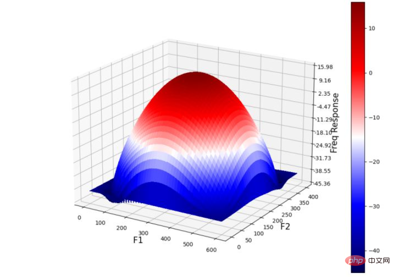
plt.show()(8) 在 3D 空间中绘制高斯核的频率响应,并使用 plot_3d() 函数:
Y = np.arange(freq.shape[0]) #-freq.shape[0]//2,freq.shape[0]-freq.shape[0]//2)
X = np.arange(freq.shape[1]) #-freq.shape[1]//2,freq.shape[1]-freq.shape[1]//2)
X, Y = np.meshgrid(X, Y)
Z = (20*np.log10( 0.01 + fp.fftshift(freq_kernel))).real
plot_3d(X,Y,Z)
下图显示了 3D 空间中高斯 LPF 核的功率谱:
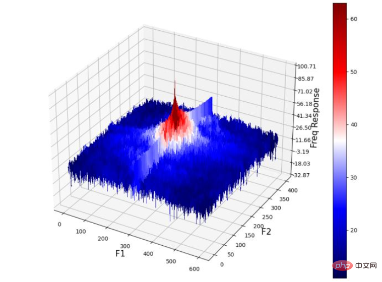
(9) 绘制 3D 空间中输入图像的功率谱:
Z = (20*np.log10( 0.01 + fp.fftshift(freq))).real
plot_3d(X,Y,Z)
(10) 最后,绘制输出图像的功率谱(通过将高斯核与输入图像卷积获得):
Z = (20*np.log10( 0.01 + fp.fftshift(convolved))).real
plot_3d(X,Y,Z)
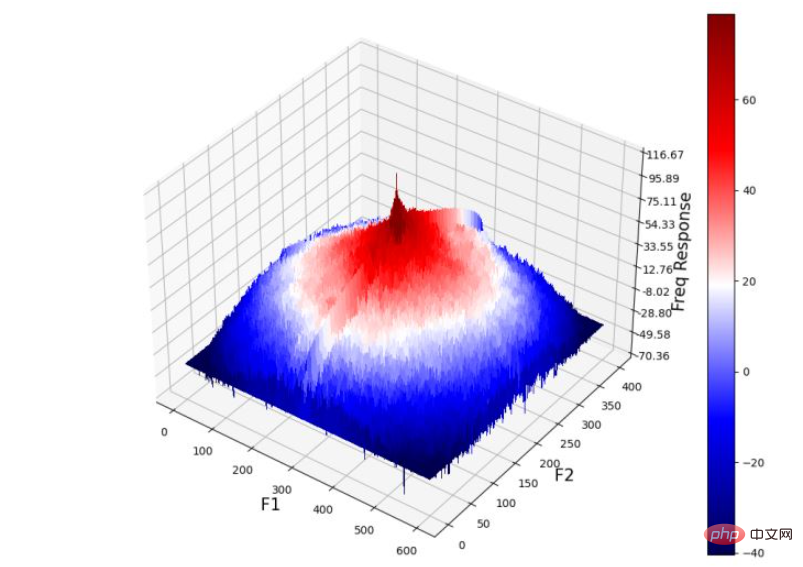
从输出图像的频率响应中可以看出,高频组件被衰减,从而导致细节的平滑/丢失,并导致输出图像模糊。
在本节中,我们将学习使用 scipy.signal 模块的 fftconvolve() 函数,用于与 RGB 彩色输入图像进行频域卷积,从而生成 RGB 彩色模糊输出图像:
scipy.signal.fftconvolve(in1, in2, mode='full', axes=None)
函数使用 FFT 卷积两个 n 维数组 in1 和 in2,并由 mode 参数确定输出大小。卷积模式 mode 具有以下类型:
输出是输入的完全离散线性卷积,默认情况下使用此种卷积模式
输出仅由那些不依赖零填充的元素组成,in1 或 in2 的尺寸必须相同
输出的大小与 in1 相同,并以输出为中心
接下来,我们实现高斯低通滤波器并使用 Laplacian 高通滤波器执行相应操作。
(1) 首先,导入所需的包,并读取输入 RGB 图像:
from skimage import img_as_float
from scipy import signal
import numpy as np
import matplotlib.pyplot as plt

im = img_as_float(plt.imread('1.png'))
(2) 实现函数 get_gaussian_edge_kernel(),并根据此函数创建一个尺寸为 15x15 的高斯核:
def get_gaussian_edge_blur_kernel(sigma, sz=15):
    # First create a 1-D Gaussian kernel
    x = np.linspace(-10, 10, sz)
    kernel_1d = np.exp(-x**2/sigma**2)
    kernel_1d /= np.trapz(kernel_1d) # normalize the sum to 1.0
    # create a 2-D Gaussian kernel from the 1-D kernel
    kernel_2d = kernel_1d[:, np.newaxis] * kernel_1d[np.newaxis, :]
    return kernel_2d
kernel = get_gaussian_edge_blur_kernel(sigma=10, sz=15)(3) 然后,使用 np.newaxis 将核尺寸重塑为 15x15x1,并使用 same 模式调用函数 signal.fftconvolve():
im1 = signal.fftconvolve(im, kernel[:, :, np.newaxis], mode='same')
im1 = im1 / np.max(im1)
在以上代码中使用的 mode='same',可以强制输出形状与输入阵列形状相同,以避免边框效应。
(4) 接下来,使用 laplacian HPF 内核,并使用相同函数执行频域卷积。需要注意的是,我们可能需要缩放/裁剪输出图像以使输出值保持像素的浮点值范围 [0,1] 内:
kernel = np.array([[0,-1,0],[-1,4,-1],[0,-1,0]])
im2 = signal.fftconvolve(im, kernel[:, :, np.newaxis], mode='same')
im2 = im2 / np.max(im2)
im2 = np.clip(im2, 0, 1)
(5) 最后,绘制输入图像和使用卷积创建的输出图像。
plt.figure(figsize=(20,10))
plt.subplot(131), plt.imshow(im), plt.axis('off'), plt.title('original image', size=10)
plt.subplot(132), plt.imshow(im1), plt.axis('off'), plt.title('output with Gaussian LPF', size=10)
plt.subplot(133), plt.imshow(im2), plt.axis('off'), plt.title('output with Laplacian HPF', size=10)
plt.tight_layout()
plt.show()
以上是Python怎麼實現低通濾波器模糊影像功能的詳細內容。更多資訊請關注PHP中文網其他相關文章!