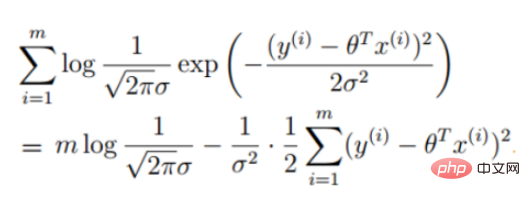
#似然函數的定義:給定聯合樣本值X下關於(未知)參數
的函數
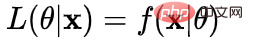

似然函數:什麼樣本的參數跟我們的資料組合後面剛好是真實值
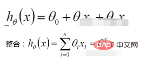
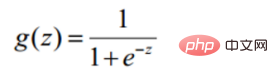 1.邏輯迴歸函數
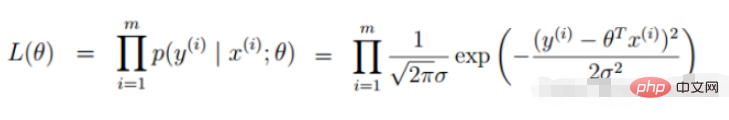
##2.邏輯迴歸似然函數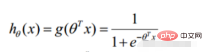
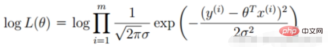
對數似然: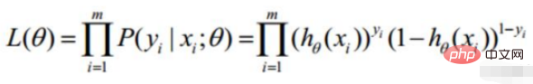
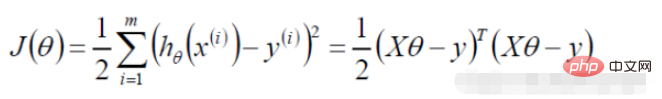
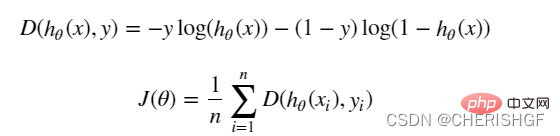
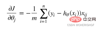
引入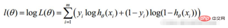 轉變為梯度下降任務,邏輯迴歸目標函數
梯度下降法解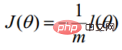
def sigmoid(z): return 1 / (1 + np.exp(-z))
def model(X, theta): return sigmoid(np.dot(X, theta.T))
##
def cost(X, y, theta): left = np.multiply(-y, np.log(model(X, theta))) right = np.multiply(1 - y, np.log(1 - model(X, theta))) return np.sum(left - right) / (len(X))
##lili 月函數
def gradient(X, y, theta): grad = np.zeros(theta.shape) error = (model(X, theta)- y).ravel() for j in range(len(theta.ravel())): #for each parmeter term = np.multiply(error, X[:,j]) grad[0, j] = np.sum(term) / len(X) return grad
梯度下降停止策略
STOP_ITER = 0 STOP_COST = 1 STOP_GRAD = 2 def stopCriterion(type, value, threshold): # 设定三种不同的停止策略 if type == STOP_ITER: # 设定迭代次数 return value > threshold elif type == STOP_COST: # 根据损失值停止 return abs(value[-1] - value[-2]) < threshold elif type == STOP_GRAD: # 根据梯度变化停止 return np.linalg.norm(value) < threshold
樣本重新洗牌
import numpy.random #洗牌 def shuffleData(data): np.random.shuffle(data) cols = data.shape[1] X = data[:, 0:cols-1] y = data[:, cols-1:] return X, y
梯度下降求解
def descent(data, theta, batchSize, stopType, thresh, alpha): # 梯度下降求解 init_time = time.time() i = 0 # 迭代次数 k = 0 # batch X, y = shuffleData(data) grad = np.zeros(theta.shape) # 计算的梯度 costs = [cost(X, y, theta)] # 损失值 while True: grad = gradient(X[k:k + batchSize], y[k:k + batchSize], theta) k += batchSize # 取batch数量个数据 if k >= n: k = 0 X, y = shuffleData(data) # 重新洗牌 theta = theta - alpha * grad # 参数更新 costs.append(cost(X, y, theta)) # 计算新的损失 i += 1 if stopType == STOP_ITER: value = i elif stopType == STOP_COST: value = costs elif stopType == STOP_GRAD: value = grad if stopCriterion(stopType, value, thresh): break return theta, i - 1, costs, grad, time.time() - init_time
import numpy as np import pandas as pd import matplotlib.pyplot as plt import os import numpy.random import time def sigmoid(z): return 1 / (1 + np.exp(-z)) def model(X, theta): return sigmoid(np.dot(X, theta.T)) def cost(X, y, theta): left = np.multiply(-y, np.log(model(X, theta))) right = np.multiply(1 - y, np.log(1 - model(X, theta))) return np.sum(left - right) / (len(X)) def gradient(X, y, theta): grad = np.zeros(theta.shape) error = (model(X, theta) - y).ravel() for j in range(len(theta.ravel())): # for each parmeter term = np.multiply(error, X[:, j]) grad[0, j] = np.sum(term) / len(X) return grad STOP_ITER = 0 STOP_COST = 1 STOP_GRAD = 2 def stopCriterion(type, value, threshold): # 设定三种不同的停止策略 if type == STOP_ITER: # 设定迭代次数 return value > threshold elif type == STOP_COST: # 根据损失值停止 return abs(value[-1] - value[-2]) < threshold elif type == STOP_GRAD: # 根据梯度变化停止 return np.linalg.norm(value) < threshold # 洗牌 def shuffleData(data): np.random.shuffle(data) cols = data.shape[1] X = data[:, 0:cols - 1] y = data[:, cols - 1:] return X, y def descent(data, theta, batchSize, stopType, thresh, alpha): # 梯度下降求解 init_time = time.time() i = 0 # 迭代次数 k = 0 # batch X, y = shuffleData(data) grad = np.zeros(theta.shape) # 计算的梯度 costs = [cost(X, y, theta)] # 损失值 while True: grad = gradient(X[k:k + batchSize], y[k:k + batchSize], theta) k += batchSize # 取batch数量个数据 if k >= n: k = 0 X, y = shuffleData(data) # 重新洗牌 theta = theta - alpha * grad # 参数更新 costs.append(cost(X, y, theta)) # 计算新的损失 i += 1 if stopType == STOP_ITER: value = i elif stopType == STOP_COST: value = costs elif stopType == STOP_GRAD: value = grad if stopCriterion(stopType, value, thresh): break return theta, i - 1, costs, grad, time.time() - init_time def runExpe(data, theta, batchSize, stopType, thresh, alpha): # import pdb # pdb.set_trace() theta, iter, costs, grad, dur = descent(data, theta, batchSize, stopType, thresh, alpha) name = "Original" if (data[:, 1] > 2).sum() > 1 else "Scaled" name += " data - learning rate: {} - ".format(alpha) if batchSize == n: strDescType = "Gradient" # 批量梯度下降 elif batchSize == 1: strDescType = "Stochastic" # 随机梯度下降 else: strDescType = "Mini-batch ({})".format(batchSize) # 小批量梯度下降 name += strDescType + " descent - Stop: " if stopType == STOP_ITER: strStop = "{} iterations".format(thresh) elif stopType == STOP_COST: strStop = "costs change < {}".format(thresh) else: strStop = "gradient norm < {}".format(thresh) name += strStop print("***{}\nTheta: {} - Iter: {} - Last cost: {:03.2f} - Duration: {:03.2f}s".format( name, theta, iter, costs[-1], dur)) fig, ax = plt.subplots(figsize=(12, 4)) ax.plot(np.arange(len(costs)), costs, 'r') ax.set_xlabel('Iterations') ax.set_ylabel('Cost') ax.set_title(name.upper() + ' - Error vs. Iteration') return theta path = 'data' + os.sep + 'LogiReg_data.txt' pdData = pd.read_csv(path, header=None, names=['Exam 1', 'Exam 2', 'Admitted']) positive = pdData[pdData['Admitted'] == 1] negative = pdData[pdData['Admitted'] == 0] # 画图观察样本情况 fig, ax = plt.subplots(figsize=(10, 5)) ax.scatter(positive['Exam 1'], positive['Exam 2'], s=30, c='b', marker='o', label='Admitted') ax.scatter(negative['Exam 1'], negative['Exam 2'], s=30, c='r', marker='x', label='Not Admitted') ax.legend() ax.set_xlabel('Exam 1 Score') ax.set_ylabel('Exam 2 Score') pdData.insert(0, 'Ones', 1) # 划分训练数据与标签 orig_data = pdData.values cols = orig_data.shape[1] X = orig_data[:, 0:cols - 1] y = orig_data[:, cols - 1:cols] # 设置初始参数0 theta = np.zeros([1, 3]) # 选择的梯度下降方法是基于所有样本的 n = 100 runExpe(orig_data, theta, n, STOP_ITER, thresh=5000, alpha=0.000001) runExpe(orig_data, theta, n, STOP_COST, thresh=0.000001, alpha=0.001) runExpe(orig_data, theta, n, STOP_GRAD, thresh=0.05, alpha=0.001) runExpe(orig_data, theta, 1, STOP_ITER, thresh=5000, alpha=0.001) runExpe(orig_data, theta, 1, STOP_ITER, thresh=15000, alpha=0.000002) runExpe(orig_data, theta, 16, STOP_ITER, thresh=15000, alpha=0.001) from sklearn import preprocessing as pp # 数据预处理 scaled_data = orig_data.copy() scaled_data[:, 1:3] = pp.scale(orig_data[:, 1:3]) runExpe(scaled_data, theta, n, STOP_ITER, thresh=5000, alpha=0.001) runExpe(scaled_data, theta, n, STOP_GRAD, thresh=0.02, alpha=0.001) theta = runExpe(scaled_data, theta, 1, STOP_GRAD, thresh=0.002 / 5, alpha=0.001) runExpe(scaled_data, theta, 16, STOP_GRAD, thresh=0.002 * 2, alpha=0.001) # 设定阈值 def predict(X, theta): return [1 if x >= 0.5 else 0 for x in model(X, theta)] # 计算精度 scaled_X = scaled_data[:, :3] y = scaled_data[:, 3] predictions = predict(scaled_X, theta) correct = [1 if ((a == 1 and b == 1) or (a == 0 and b == 0)) else 0 for (a, b) in zip(predictions, y)] accuracy = (sum(map(int, correct)) % len(correct)) print('accuracy = {0}%'.format(accuracy))
#形式簡單,模型的可解釋性非常好。從特徵的權重可以看到不同的特徵對最後結果的影響,某個特徵的權重值比較高,那麼這個特徵最後對結果的影響會比較大。
模型效果不錯。在工程上是可以接受的(作為baseline),如果特徵工程做的好,效果不會太差,並且特徵工程可以大家並行開發,大大加快開發的速度。
訓練速度較快。分類的時候,計算量僅僅只和特徵的數目相關。且邏輯迴歸的分散式最佳化sgd發展比較成熟,訓練的速度可以透過堆機器進一步提高,這樣我們可以在短時間內迭代好幾個版本的模型。
資源佔用小,尤其是記憶體。因為只需要儲存各個維度的特徵值。
方便輸出結果調整。邏輯迴歸可以很方便的得到最後的分類結果,因為輸出的是每個樣本的機率分數,我們可以很容易的對這些機率分數進行cutoff,也就是劃分閾值(大於某個閾值的是一類,小於某個閾值的是一類)。
準確率不是很高。因為形式非常的簡單(非常類似線性模型),很難去擬合資料的真實分佈。
很難處理資料不平衡的問題。舉個例子:如果我們對於一個正負樣本非常不平衡的問題例如正負樣本比 10000:1.我們把所有樣本都預測為正也能讓損失函數的值比較小。但是作為一個分類器,它對正負樣本的區分能力不會很好。
處理非線性資料較麻煩。邏輯迴歸在不引入其他方法的情況下,只能處理線性可分的數據,或者進一步說,處理二分類的問題 。
邏輯迴歸本身無法篩選特徵。有時候,我們會用gbdt來篩選特徵,然後再上邏輯回歸。
以上是python如何實現梯度下降求解邏輯迴歸的詳細內容。更多資訊請關注PHP中文網其他相關文章!